Validation

How well a theoretical simulation needs to model the helicopter behaviour depends very much on the application; in the simulation world the measure of quality is described as the fidelity or validation level. Fidelity is normally judged by comparison with test data, both model and full scale. The validation process can be described in terms of two kinds of fidelity-functional and physical (Ref. 2.19), defined as follows:

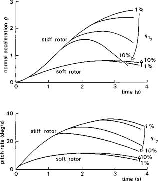
Fig. 2.31 Nonlinear pitch response for Lynx at 100 knots

Functional fidelity is the level of fidelity of the overall model to achieve compliance with some functional requirement, e. g., for our application, can the model be used to predict flying qualities parameters?

Physical fidelity is the level of fidelity of the individual modelling assumptions in the model components, in terms of their ability to represent the underlying physics, e. g., does the rotor aerodynamic inflow formulation capture the fluid mechanics of the wake correctly?

It is convenient and also useful to distinguish between these two approaches because they focus attention on the two ends of the problem – have we modelled the physics correctly and does the pilot perceive that the simulation ‘feels’ right? It might be imagined that the one would follow from the other and while this is true to an extent, it is also true that simulation models will continue to be characterized by a collection of aerodynamic and structural approximations, patched together and each correct over a limited range, for the foreseeable future. It is also something of a paradox that the conceptual product of complexity and physical understanding can effectively be constant in simulation. The more complex the model becomes, then while the model fidelity may be increasing, the ability to interpret cause and effect and hence gain physical understanding of the model behaviour diminishes. Against this stands the argument that, in general, only through adding complexity can fidelity be improved. A general rule of thumb is that the model needs to be only as complex as the fidelity requirements dictate; improvements beyond this are generally not cost-effective. The problem is that we typically do not know how far to go at the initial stages of a model

development, and we need to be guided by the results of validation studies reported in the literature. The last few years have seen a surge of activity in this research area, with the techniques of system identification underpinning practically all the progress (Refs 2.20-2.22). System identification is essentially a process of reconstructing a simulation model structure and associated parameters from experimental data. The techniques range from simple curve fitting to complex statistical error analysis, but have been used in aeronautics in various guises from the early days of data analysis (see the work of Shinbrot in Ref. 2.23). The helicopter presents special problems to system identification, but these are nowadays fairly well understood, if not always accounted for, and recent experience has made these techniques much more accessible to the helicopter flight dynamicist.

An example illustrating the essence of system identification can be drawn from the roll response dynamics described earlier in this chapter; if we assume the first-order model structure, then the equation of motion and measurement equation take the form

P — Lpp — L&ic ®lc + Ep (2 73)

P = f (Pm) + Em

The second equation is included to show that in most cases, we shall be considering problems where the variable or state of interest is not the same as that measured; there will generally be some measurement error function Em and some calibration function f involved. Also, the equation of motion will not fully model the situation and we introduce the process error function ep. Ironically, it is the estimation of the characteristics of these error or noise functions that has motivated the development of a significant amount of the system identification methodology.

The solution for roll rate can be written in either a form suitable for forward (numerical) integration

t

P = P0 + / (LpP(r) + L вс °ic (t ))dT (2.74)

0

or an analytic form

t

p — poeLpt + j eLp(t-t)Lelc91c(t)dT (2.75)

0

The identification problem associated with eqns 2.73 becomes, ‘from flight test mea­surements of roll rate response to a measured lateral cyclic input, estimate values of the damping and control sensitivity derivatives Lp and Le1c ’. In starting at this point, we are actually skipping over two of the three subprocesses of system identification – state estimation and model structure estimation, processes that aim to quantify bet­ter the measurement and process noise. There are two general approaches to solving the identification problem – equation error and output error. With the equation error method, we work with the first equation of 2.73, but we need measurements of both roll rate and roll acceleration, and rewrite the equation in the form

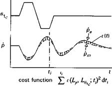
Fig. 2.32 Equation error identification process

Subscripts m and e denote measurements and estimated states respectively. The identi­fication process now involves achieving the best fit between the estimated roll acceler­ation pe from eqn 2.76 and the measured roll acceleration pm, varying the parameters Lp and Lo1c to achieve the fit (Fig. 2.32). Equation 2.76 will yield one-fit equation for each measurement point, and hence with n measurement times we have two unknowns and n equations – the classic overdetermined problem. In matrix form, the n equations can be combined in the form

x = By + e (2.77)

where x is the vector of acceleration measurements, B is the (n x 2) matrix of roll rate and lateral cyclic measurements and y is the vector of unknown derivatives L p and Lo1c; e is the error vector function. Equation 2.77 cannot be inverted in the conventional manner because the matrix B is not square. However, a pseudo-inverse can be defined that will provide the so-called least-squares solution to the fitting process, i. e., the error function is minimized so that the sum of the squares of the error between, measured and estimated acceleration is minimized over a defined time interval. The least-squares solution is given by

y = (BTB)-1BTx (2.78)

Provided that the errors are randomly distributed with a normal distribution and zero mean, the derivatives so estimated from eqn 2.78 will be unbiased and have high confidence factors.

The second approach to system identification is the output error method, where the starting equation is the solution or ‘output’ of the equation of motion. In the present example, either the analytic (eqn 2.74) or numerical (eqn 2.73) solution can be used; it is usually more convenient to work with the latter, giving the estimated roll rate in this case as

t

pe = P0m + J (Lp Pm (T) + L Ole Oicm (T ))dT (2.79)

0

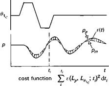
Fig. 2.33 Output error identification process

The error function is then formed from the difference between the measured and estimated roll rate, which can once again be minimized in a least-squares sense across the time history to yield the best estimates of the damping and control derivatives (Fig. 2.33).

Provided that the model structures are correct, the processes we have described will always yield ‘good’ derivative estimates in the absence of ‘noise’, assuming that enough measurements are available to cover the frequencies of interest; in fact, the two methods are equivalent in this simple case. Most identification work with simulated data falls into this category, and new variants of the two basic methods are often tested with simulation data prior to being applied to test data. Without contamination with a realistic level of noise, simulation data can give a very misleading impression of the robustness level of system identification methods applied to helicopters. Expanding on the above, we can classify noise into two sources for the purposes of the discussion:

(1) measurement noise, appearing on the measured signals;

(2) process noise, appearing on the response outputs, reflecting unmodelled effects.

It can be shown (Ref. 2.24, Klein) that results from equation error methods are suscep­tible to measurement noise, while those from output error analysis suffer from process noise. Both can go terribly wrong if the error sources are deterministic and cannot therefore be modelled as random noise. An approach that purports to account for both error sources is the so-called maximum likelihood technique, whereby the output error method is used in conjunction with a filtering process, that calculates the error functions iteratively with the model parameters.

Identifying stability and control derivatives from flight test data can be used to provide accurate linear models for control law design or in the estimation of handling qualities parameters. Our principal interest in this Tour is the application to simulation model validation. How can we use the estimated parameters to quantify the levels of modelling fidelity? The difficulty is that the estimated parameters are made up of contributions from many different elements, e. g., main rotor and empennage, and the process of isolating the source of a deficient force or moment prediction is not obvious. Two approaches to tackling this problem are described in Ref. 2.25; one where the model parameters are physically based and where the modelling element of interest is isolated from the other components through prescribed dynamics – the so-called open-loop or constrained method. The second method involves establishing the relationship between the derivatives and the physical rotorcraft parameters, hence enabling the degree of distortion of the physical parameters required to match the test data. Both these methods are useful and have been used in several different applications over the last few years.

Large parameter distortions most commonly result from one of two sources in helicopter flight dynamics, both related to model structure deficiencies – missing DoFs or missing nonlinearities, or a combination of both. A certain degree of model structure mismatch will always be present and will be reflected in the confidence values in the estimated parameters. Large errors can, however, lead to unrealistic values of some parameters that are effectively being used to compensate for the missing parts. Knowing when this is happening in a particular application is part of the ‘art’ of system identification. One of the keys to success involves designing an appropriate test input that ensures that the model structure of interest remains valid in terms of frequency and amplitude, bringing us back to the two characteristic dimensions of modelling. A relatively new technique that has considerable potential in this area is the method of inverse simulation.