COMPUTATION OF THE ROBUST DELAY MARGIN

The aim of this subsection is to present the principle of the method in a qualitative way: see the following section for a detailed algorithm.

•LetM(s)- A(s) the standard interconnection structure, with Д(в) = diag(Ai(s), A2(s)). Remember Ai(s) is a mixed model perturbation gathering all classical model uncertainties, whereas Дг(а) gathers all un­certain time delays (see equation (11.4)).

Assuming that the nominal closed loop (i. e. the closed loop without time delays and model uncertainties) is asymptotically stable and with reference to the Nyquist stability criterion (Ferreres and Scorletti, 1998), the key point is to note that the analysis of the robust stability property of the closed loop reduces to the problem of detecting at each frequency и the singularity of the matrix I — M(juj)A(ju), i. e.:

det(I – M{jw)diag{A(ju),e~^UTl – 1,… ,e~j“TN – 1) = 0 (11.7)

The frequency u> is fixed in the following, and the w dependence is drop out, so that M and Д = diag(Aі, Д2) mean the values of M(s) and Д($) = diag(Ai(s), Д2(я)) at s = ju>.

constraint (e. g. |<5гс| < 1). This explains why conservative results are obtained with this method, even if the exact value of /л is computed.

In order to fully take into account this information and with reference to the bilinear transformation, the idea is simply to rewrite the complex

scalars S£ ’ s as:

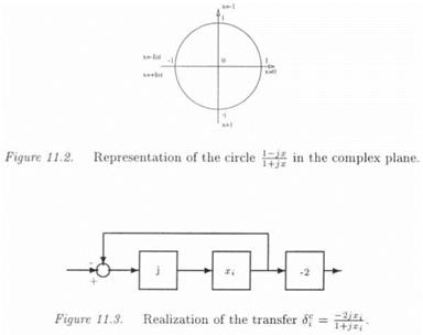
where j2 — — 1 and the real scalar хг belongs to the interval [—oo, +oo] (see Figure 11.2). The magnitude of 1 + Sf is now constrained to be 1, and a real scalar X{ is to be handled. Sf is thus (see also Figure 11.3 for an LFT realization):

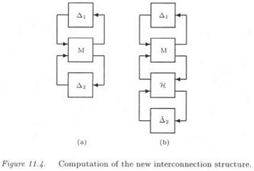
• We come back to the initial interconnection structure M – Д, with Д = diag(Aі, Д2). With reference to equations (11.8) and (11.10), each complex scalar S is rewritten as an LFT Fi(H, Xi), with:

In the same way, the model perturbation Д s is rewritten as 2),

where:

Д2 = diag{xi,…,xN)

As a consequence, the initial interconnection structure Д – Д of Fig­ure 11.4.a can be transformed into the new equivalent interconnection structure M—A of Figure 11.4.b, where M = M[12]H and A = diag(A 1, A2) (see subsection 3.1 of chapter 3 for the definition of the star product M-kH). The interconnection of LFTs is indeed an LFT.

Remark: consider the problem of checking whether a template on a closed loop transfer function remains satisfied despite classical model uncertainties (parametric uncertainties and neglected dynamics). Fol­lowing chapter 1 (section 4.4), this classical robust performance prob­lem can be converted into an augmented stability problem, in which a full complex block is added to the structured model perturbation. As a consequence, the method described in this section can be extended to the problem of checking whether a template on a closed loop trans­fer function remains satisfied despite parametric uncertainties, neglected dynamics and delays.