Our heavyweight helicopter equal in the world does not have
In Rostov started production of the most load-lifting rotary-wing car The Russian holding «Helicopt[...]

Everything about aircrafts and helicopters. News and events in aviation worldwide. Civil, transportation, military helicopters and airplanes.

Everything about aircrafts and helicopters. News and events in aviation worldwide. Civil, transportation, military helicopters and airplanes.

Everything about aircrafts and helicopters. News and events in aviation worldwide. Civil, transportation, military helicopters and airplanes.

Everything about aircrafts and helicopters. News and events in aviation worldwide. Civil, transportation, military helicopters and airplanes.


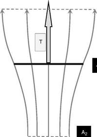
In modelling the actuator disc in descent, the air enters the streamtube from below the rotor with velocity VD and then acquires a reduction in velocity of V as it passes through the rotor disc. It finally forms the wake with a velocity decrease of V2. In this situation, the upward-going air has its velocity reduced as it passes along the streamtube from below the rotor to above the rotor where the wake forms. This is an effective increase in downward momentum of the air and this is how an upward thrust force can be generated from upward-moving air. The situation is shown in Figures 2.11-2.13.
|
|
|
|
|
|
The rotor thrust force, T, can be evaluated by considering this momentum increase. With reference to Figures 2.11 and 2.12, the continuity of the flow through the streamtube can be expressed thus:
pAi (Vd-V2) = pA(VD-Vi) = M2(Vd) (2.36)
The rate of change of momentum gives the rotor thrust as:
T = pA(VD-Vi)V2 (2.37)
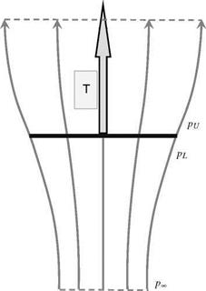
The thrust can also be expressed in terms of the difference of air pressure on both sides of the rotor disc – see Figure 2.13 – where we have the following:
T = A(pl-Pu) (2.38)
As before, Bernoulli’s equation can be applied to the flow above or below the rotor disc, but not through it. Above the rotor we have:
while below the rotor:
![]() Pl + 2 P(Vd—vi)2 = Pi + 2 P(Vd)2
Pl + 2 P(Vd—vi)2 = Pi + 2 P(Vd)2
 |
||
Subtracting these gives:
Assembling (2.37), (2.38) and (2.41) gives the same result as in climb/hover, namely:
V2 = 2Vi (2.42)
from which we obtain from (2.37):
T = 2pA(Vd—Vi) Vi (2.43)
The streamtube modelling which was conducted for climb is now directed at descent. For the descent case, the velocity variation down the length of the streamtube again can be defined
relatively simply thus:
V = Vd-V + Vi • tanh(k0 (2.44)
where the terms are as used in the climb case (s is still positive downward).
The pressure variation now becomes as follows.
Above rotor:
Pi+ 1 P(VD-2Vi)2 = p + 2 PV
![]() P-Pi _ (Vd-2Vi)2—V2 P 2
P-Pi _ (Vd-2Vi)2—V2 P 2
Below rotor:
![]() (2.46)
(2.46)
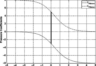
Using the pressure coefficient, based on the reference air velocity of U, we find the following results for the pressure variation for above the rotor (CPU) and below the rotor (CPL):
![]() (VD-2Vi)2-V2 Cpu = —U—
(VD-2Vi)2-V2 Cpu = —U—
C _(Vd)2-V2 Cpl = U2
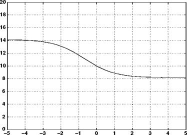
With a descent velocity of 30 m/s, an induced velocity of 10 m/s and a rotor radius of 10 m, the velocity, streamtube size and the pressure variation with axial location are as shown in Figures 2.14-2.16.
The results are similar to the climb case and the pressure jump required to generate the rotor thrust is again shown.
An examination of these two analyses might appear to give the impression that descent and climb are closely matched and that there would be no reason to foresee any difficulties. The analyses are beguiling. The sting in the tail is that actuator disc theory assumes a onedimensional and incompressible flow. Therefore the flow direction must not change throughout the entire length of the streamtube – the constant mass flow guarantees this. In climb it must always be downward. For climb, Equation 2.32 guarantees this will happen. However, for descent, Equation 2.44 admits the possibility of a flow reversal. This begins to define the problems which are faced in modelling the lower descent rate of a helicopter rotor.
To see the potential problem, recall Equations 2.26 and 2.43. Collating the results and substituting to remove V2 terms we find the following.
Climb/hover:
|
Above Rotor – Streamtube Location – Below Rotor Figure 2.14 Axial velocity variation
|
|
|
|
|
|
|
|
![]() T = 2A • p(VD-Vi)Vi
T = 2A • p(VD-Vi)Vi
If we now set the value of the climb/descent velocity to zero the situation of hover is achieved. Remembering that we denote the hovering induced velocity by V0, (2.48) and (2.49) become:
![]() T = 2pA •
T = 2pA •
T = -2pA •
The upper (climb) equation produces a relationship which sensibly defines the hovering induced velocity as:
The second descent equation produces a conflict. The thrust force is always upward and must, therefore, always have a positive value. This cannot happen with this equation. This is an indication of a problem with actuator disc theory in descent – it cannot be extended to hover, leaving a domain which this equation cannot model. As will be seen, the theory works for
appropriate values of descent rate but, as just described, it cannot be extended back to the hovering condition.
Combining the results (2.51) with (2.48) and (2.49) gives:
![]() = 2ТЇ =(Vc + V)V
= 2ТЇ =(Vc + V)V
V2 = IpA = (Vd-V)V
If we define the following normalized velocity terms:
and make the subst tut on:
![]() Vd = – Vc
Vd = – Vc
(so that both climb and descent use a common velocity sign convention), we obtain the following non-dimensional equations:
(Vc + Vi) Vi = 1
(Vc + Vi )V =-1
Equations 2.55 are then solved to give solutions for the induced velocity; however, only positive solutions are physically appropriate. A simple interpretation of these solutions can be obtained by re-expressing Equations 2.55 as:
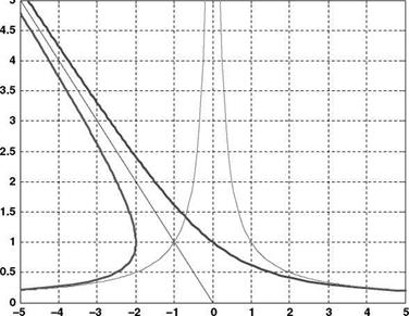
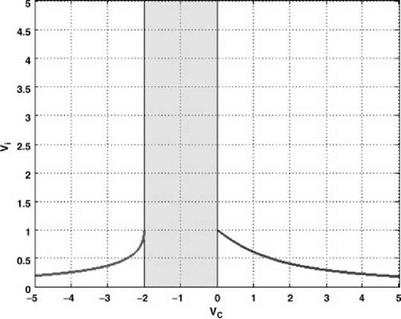
Vc =± V – Vi (2.56)
These represent the sum of a rectified rectangular hyperbola and a linear function as shown in Figure 2.17.
There is the requirement for the air to flow in one direction only (which was introduced earlier), and in order to satisfy this condition, limitations on the solutions must be made. Observation of the solutions shows that in order for the flow to be in the same direction at the entry, rotor disc and exit cross-sections of the streamtube, a region of axial velocity must be removed as shown in Figure 2.18.
![]()
|
|
|
Where the limits on the vertical velocity are those which give a real mathematical solution, Equation 2.55 now becomes:
![]() (VC + Vi) Vi = 1 , Vc > 0 (VC + Vi)V =-1 , VC <-2
(VC + Vi) Vi = 1 , Vc > 0 (VC + Vi)V =-1 , VC <-2
It is therefore necessary to seek alternative solutions to the conditions experienced in this region. While this is relatively easy to write down, it is very difficult to handle theoretically. This is because the actuator disc relies on a definable streamtube while the flow conditions in the nonqualifying region are not in any way conducive to such a concept. Indeed, the actual situation isof a system of vortices being generated by the lifting rotor blades and becoming the dominant feature. In axial descent, at low speed, the downwash induced by the rotor and wake is matched by the upward motion induced by the descending rotor, resulting in the vorticity in the wake remaining in close proximity to the rotor disc. It is reasonable to observe that the rotor cannot store vorticity for ever and so there must some manner in which itcan disperse. In reality ittends to collect around the rotor giving rise to difficulties in handling and to act as a source of high – frequency vibration. Periodically, this collected vorticity releases, freeing up the rotor, whence the process can start again. This will contribute to the vibration by adding a low-frequency component to the previously mentioned high frequency. As can be envisaged, the airflow characteristics of a helicopter rotor, in what is termed the vortex ring state, are very complex and difficult flow conditions to model theoretically and have exercised many minds over the years.
Although these flight conditions are complex, it is instructive to consider what the mean flow behaviour would be. This directs the discussion to the various flow states that a helicopter rotor can experience as it moves from high-rate vertical climb to high-rate vertical descent.
These are presented schematically in Table 2.1.