DRP Scheme in Curvilinear Coordinates

Most practical computations are often not carried out in Cartesian coordinates. Instead, the actual computations usually are done on a set of body-fitted curvilinear coordinates. Thus, the space of the curvilinear coordinate system forms the com­putation domain. In other words, the governing equations, written in curvilinear coordinates, will be discretized and computed. It will be shown that, if the optimized spatial and temporal discretization method developed in Chapters 2 and 3 are used, then the discretized equations retain the DRP property.

The three-dimensional compressible Euler equations for a perfect gas in Carte­sian coordinates may be written as

d u 9 u „ 9 u

—– + A—— + B—

dt dx dy

where

p		u	p	0	0	0		v	0	p	0	0		w	0	0	p	0
u		0	u	0	0	1 P		0	v	0	0	0		0	w	0	0	0
v	A=	0	0	u	0	0	B=	0	0	v	0	1 p	C=	0	0	w	0	0
w		0	0	0	u	0		0	0	0	v	0		0	0	0	w	1 p
_p_		0	Y P	0	0	u		0	0	Yp	0	v		0	0	0	Yp	w

Now, let f (x, y, z), n(x, y, z), and Z (x, y, z) be a set of curvilinear coordinates. This set of coordinates will be used for discretizing the Euler equations and for computing the solution. A simple change of variables by means of the chain rule transforms Eq. (5.60) into an equation with (f, n, Z) as independent variables in the following form:

where

A = df A+df B + df c

dx dy dz

B = —a + A B + Ac

dx dy dz

c = A – A + a B + A c.

dx dy dz

Suppose the Fourier-Laplace transform of a function/(f, n, Z, t) is /(а, в, Y,«) and that of

(5.62)

By means of convolution interal (5.62), the Fourier-Laplace transform of the Euler equation (5.6i) may be written as follows:

+ i^B(a — ai, в — во Y — Yi, a — ai) + i’YiC(a — ai, в — во Y — Yi, a — ai)] x ii(ai, в1, Yi, ai) dai dв1 dYi dai.

Now, for the purpose of computation, let Eq. (5.6i) be discretized in the (f, n, Z) spacing using the 7-point stencil optimized scheme and the four-level time march­ing algorithm developed in Chapters 2 and 3. The discretized equations are as follows:

j=0

The Fourier-Laplace transforms of the discretized Eqs. (5.64) and (5.65) are

— ai, в — ві, Y — Уі, « — «і) + i У(Уі)C(a — аі, в — ві, Y — Уі, « — «і)]

x й(аі, ві, Y!, «і) da1 dв1 dY1 й«і – (5.67)

Upon eliminating Ё from Eqs. (5.66) and (5.67), the Fourier-Laplace transform of the discretized solution is given by

аі, в — ві, Y — Уі, « — «і)

+ i в(ві)B(a — аі, в — ві, Y — Уі, « — «і)•

+ i У(Уі)C(a — аі, в — ві, Y — Уі,« — «і)] x й(аі, ві, Y^ «і) dax dв1 dY1 d«v (5.68)

By comparing Eqs. (5.63) and (5.68), it becomes clear that, if the discretized solution is restricted to the range for which а(а) = а, в(в) = в, Y(y) = Y, and «(«) = «, the equations are identical. Thus, the discretized Eqs. (5.64) and (5.65) are DRP in the sense that their Fourier-Laplace transforms are formally the same as the exact solution of Euler equations.

EXERCISES

5.1. The propagation of electromagnetic waves is governed by the Maxwell equa­tions:

дє 9 Ё ———— V x B = 0 C dt	()
і 9 B	(2)
—— + Vx Ё = 0 C dt
< И II о	(3)
<1 Я II о	(4)

where Ё and B are the electric and magnetic fields and д and є are material constants. Now, look for plane wave solutions in the following form:

Ё = e E/(k’x—«(), (5)

where e is a constant unit vector characterizing the direction of the electric field. E0 is the amplitude and k = aex + в ey + у ez, where ex, ey, ez are the unit vectors in the

x, y, and z directions, is the wave vector and ш is the angular frequency. Eqs. (2) and (4) are satisfied automatically if the magnetic field is given by

c

B = – (k x E). (6)

ш

Substitution of (5) and (6) into (1) and (3) leads to

шілє~ ci /і ^

—- e = — k x (k x e)

c ш

Є ■ k = 0.

(Note: Eqs. (7) and (8) can also be obtained by taking the Fourier-Laplace transform of Eqs. (1) to (4). In this case, the transform variables are (а, в, у, ш)).

If Є = f Єх+ + пЄу + Zez is the solution of Eq. (7), then Eq. (8) is automatically satisfied. By writing Eq. (7) in a matrix form for the unknowns (f, n, Z), the disper­sion relations of electromagnetic waves are given by setting the determinant of the coefficient matrix to zero.

Discretize the Maxwell equations according to the DRP scheme. Show that the discretized equation formally preserves the dispersion relation of the electromag­netic waves; i. e., ш replaces ш, (а, в, у) replaces (а, в, у), respectively.

5.2. Consider solving the convective equation

d u d u

——- + c— = 0

dt dx

computationally by using central difference approximation. Suppose we use differ­ent size stencils; e. g., N = 7, 9, 11 etc. Assume that the same time marching scheme is used. Show that the maximum time step At allowed by numerical stability require­ment is smaller when a larger size stencil is used.

(Note: This result is not restricted to the convective equation. It is true for the solution of the Euler equations and the Maxwell equations.)

5.3. Consider solving numerically the following initial value problem:

9 u 9 u

— ^ — = t = u = f(x).

dt dx

In standard numerical analysis books, one finds that the spatial derivative may be discretized in three ways.

(a) Forward difference

+ O(Ax2)

(b) Central difference

+ O(Ax2)

(c) Backward difference

/ 9 u 9 x

1. Determine which of these finite difference schemes would lead to stable numerical solution, assuming that the time derivative is computed exactly.

2. Now apply the same discretization to the linearized Euler equations in one dimension.

du d p d p d U

—— + — = 0, — +————– = 0.

dt dx d t dx

Determine which of these schemes are suitable for solving this system of equations.

3. If the central difference scheme is used for the x derivative and the four – level time marching DRP scheme is used to advance the solution in time, determine the largest At one may use for solving the one-dimensional Euler equations.

5.4. Suppose an upwind difference

d u 3иг — 4иг_1 + U^_2

2Ax

is used to approximate the x derivative of the equation

d U d U

—– + c— = 0

d t dx

in the solution of the initial value problem

U (x, 0) = Є (1"2)[1°ax ]

By using Im(a Ax) or otherwise estimate the decrease in the area of the pulse after it has propagated over a distance of 400 mesh points. Estimate the shape of the pulse. Compare your estimate with your numerical solution.

5.5. Solve the dimensionless spherical wave problem computationally

d U U d U T – + – + T – = 0 dt x dx

over the domain 5 < x < 5 with initial condition t = 0, U = 0. The boundary condition at x = 5 is

U = sin

Here, x is nondimensionalized by Ax, U by a (the speed of propagation), and t by Ax/a. Give the numerical solution at t = 50 and 200 over the interval 150 < x < 250. Plot the result in graphical form. Compare your numerical solution with the exact solution as follows:

5 sin [4 (t — x + 5)], x < t + 5 0, x > t + 5, t — x + 5 < 0

5.6. Consider simulating the propagation and reflection of acoustic disturbance in a semiinfinite long tube with a closed end at x = 0 as shown. The governing equations are the linearized Euler equations in one dimension. On using Ax (the mesh size) as the length scale, a0 (the speed of sound) as the velocity scale, Ax/a0 as the time scale, p0a0 as the pressure scale, where p0 is the gas density inside the tube, the

dimensionless governing equations may be written as

d u d p

—— + —

dt dx 9 p d u

— +—–

dt dx

The gas is set into motion by a pressure pulse at t = 0; i. e.,

Use a computational domain 0 < x < 100; calculate the pressure and velocity distri­bution at t = 40 by a time marching scheme. Compare your solution with the exact solution as follows:

5.7.

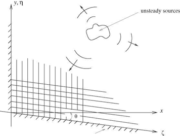To compute the sound field radiated by two-dimensional unsteady sources in the vicinity of two walls intersecting at an angle as shown in the figure below, a natural

choice is to use oblique Cartesian coordinates (f, n). (f, n) are related to Cartesian coordinates (x, y) by

x

f =——— , n = У + xsin в.

s cos в 1 7

a. Transform the governing equations (linearized Euler equations) from Carte­sian to oblique Cartesian coordinates.

b. Discretize the equations in oblique Cartesian coordinates by the use of the 7-point stencil DRP scheme.

c. Show that in the computation domain (the f – n plane) the discretized equations are dispersion-relation preserving.