Low-Rank Response Surface

Our heavyweight helicopter equal in the world does not have

In Rostov started production of the most load-lifting rotary-wing car The Russian holding «Helicopt[...]

The old plane — nonsense, pilots think - there was an attack

In spite of the fact that the main version of crash of the Russian plane of the Kogalymavia company [...]

Low-Rank Response Surface

To compute statistics of the random (uncertain) solution (error-bars, quantiles, cumulative density function, etc) accurate enough, one needs a large sample size. Monte Carlo simulations are expensive. To decrease the computational costs we compute a, so-called, response surface — (multivariate) polynomial (see Eq. 10). The idea [13] is to construct a good response surface from few samples and then
to use the residual for its improvement. A motivation for this idea comes from the fact that in many software packages for solving engineering and physical problems it is impossible or very difficult to change the code, but it is possible to access the residual. Later on the computed response surface is used for very fast generation of a large sample.

Let у(л;, в) be the solution ( or a functional of the solution). It can be pressure, density, velocity, lift, drag etc. v(x, в) can be approximated in a set of new independent Gaussian random variables (truncated polynomial chaos expansions of Wiener [25])

(x, в(ю)) « X vp(x)Hp(e) = l-vp(x)-}l-Hp(e)-]T> (10)

$Подпись: V/3(X> = -^J0Hp(e)v{x,e)¥{de)$

where coefficients vp (x) are computed as follows

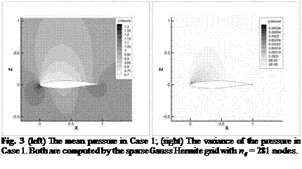
The PCE representation in Eq. 10 was used to compute the mean and the variance of the pressure (see Fig. 3) for the Case 1 (a = 1.93 and Ma = 0.676, no shock). PCE coefficients are computed by the sparse Gauss Hermite grid with nq = 281 nodes. Here the multidimensional integral over 0 is computed approximately, for example, on a sparse Gauss-Hermite grid [6, 2].

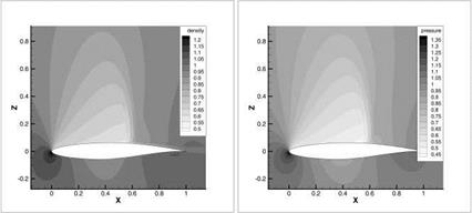
Fig. 4 demonstrates the mean of density and mean of pressure, computed again as in Eq. 10 for the Case 9 (a = 2.79 and Ma = 0.734, with shock).

Подпись: Fig. 3 (left) The mean pressure in Case 1; (right) The variance of the pressure in Case 1. Both are computed by the sparse Gauss Hermite grid with nq = 281 nodes.
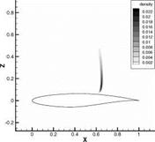
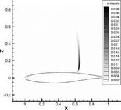
Fig. 5 demonstrates the variance of density and variance of pressure, computed via Monte Carlo methods for the Case 9. One can see the largest uncertainty in the shock position.