Comparison of Theoretical Solution to Experimental Data

It is of interest at this point to compare the analytical solution to actual experi­mental data for the laminar boundary-layer results. The problem just solved may seem rather abstract because of the several stages required in its definition. It was necessary first to derive the basic equations describing the fluid dynamics. The equations then were modified using Prandtl’s physical insights to properly incor­porate the viscous terms. This led to stretching the coordinate normal to the wall and the introduction of the boundary-layer coordinate, n. A powerful mathemat­ical technique, the similarity method, then was used to find an analytical solution. After all of this manipulation of the problem, the student may wonder if there is anything left that properly represents reality. As usual, the answers can be found

<D a 1= о о

0 0.2 0.4 0.6 0.8 1 1.2

/ я f"

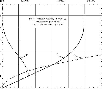
Figure 8.11a. Plots of the Blasius function, f, and its derivatives.

only by comparing analytical results to experimental measurements. This was done by many investigators, but a particularly careful set of measurements was carried out by Nikuradse in 1942 (See Thwaites, 1949). His measurements were made at five locations along the flat plate to study the effect of the Re number (in the range 1.1.105 < Re < 7.3.105) on the velocity profile. One item that he wanted to verify was the similarity of the velocity profiles. That is, the shape of the velocity distri­bution should be the same at any axial location. Figure 8.11b shows his measure­ments. The horizontal axis is the boundary-layer coordinate as we defined it in Eq. 8.46. The vertical axis in this plot is the value of the dimensionless x-velocity, f = u/Ue. There can be no question that the agreement between the Blasius flat – plate theory and the experimental data is virtually perfect. This should help to build the student’s confidence in the powerful mathematical methods introduced herein.