MATHEMATICAL MODEL OF HUMAN PILOTS — PURSUIT DISPLAY

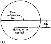Pilot models are being developed to describe the control situation when displays other than the compensatory type are utilized. An example of this is the pursuit display. The single-degree-of-freedom tracking task with a pursuit display is identical to the compensatory task of Fig. 12.3a except that the displayed variables are different—i. e. the pilot has different infor­mation. In the compensatory task only e(t) is displayed (Fig. 12.3) whereas in the pursuit task both i(t) and m(t) are separately displayed. Figure 12.6 illustrates the difference between the two displays for the same system state. It can be seen that additional information is presented to the pilot on the pursuit display. Although e(f) is available in both cases, only the pursuit display separates the error into its components and conveys this information to the pilot. For example, a pursuit display tells the pilot whether his tracking error is due to a difficult input signal, i(t), or due to erratic pilot control of the aircraft, m(t), which in turn can affect his strategy in bringing the tracking

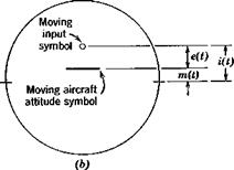Fig. 12.6 Displays, (a) Compensatory. (6) Pursuit.

error under control. Whether the one display or the other is best for the mission at hand is a complex function of the task performed.

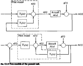A technique for measuring human-pilot describing functions has been developed for the single-degree-of-freedom tracking task with a pursuit dis­play for situations where a secondary disturbance signal is present. This task is shown in Fig. 12.7. It might for example represent a mid-air refueling task where i(t) represents the tanker’s altitude and the secondary disturbance g(t) represents turbulence acting on the controlled aircraft. The model of this task can be formulated in several ways. Figure 12.8 shows two useful forms of the model. The pilot is represented by a pair of describing functions (F2(s), Y2(s)) or (Ys(s), Yfls)) since the pilot is considered to have

two inputs and one output. [Since e(t) = i(t) — m(t) it is redundant to con­sider a case with three inputs.] Again n(t) represents the remnant. The describing function pairs are chosen to minimize the root mean square of that part of the vehicle input signal o(t) which is accounted for by n(t) (as was done for the compensatory display). The describing functions that result are [where the aircraft transfer function is A(s)]:

Гі(г’со) = (77— + A(ia>)

Г2(гш) = (1 — Y1(ico)A(ia))) ■ ф2(а>)

Y3(ia>) = Y2(ico)

Y^ico) = Y^ico) – f – Гг(т>)

where фАсо) =

Ф«(ю)Ф„(й>)-Фл(®)Ф«(«>)

__ Ф»ФИ(<») – Og0(tt))O,-g(ft>)

2 Фц(о>)Фдд(а>) — Фід(а>)ФЯі(о>)

The denominators of (12.3,1) both vanish if either (i) g(t) = 0 or (ii) g(t) = const X i(t). In either of these cases the measurement of фг and ф2, and hence of the describing function pairs, would not be possible. In addition the following are found to hold:

ФшМ = Фдп{ы) = 0

Ф0»

X {|Т’2(іса)|2фіі(й)) + І Т1(г<ы)|2Ф!,д(а)) + 2 Re [F|(*’o)) (12.3,3) X Г1(*со)фг9(с»)]}

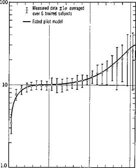
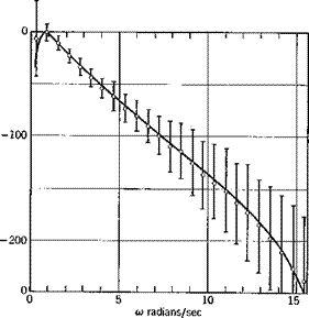
As yet no general set of rules comparable to those for the compensatory task has been developed to cover this model. A typical measured pursuit model is shown in Fig. 12.9. It was found that the measured data could be fitted quite well by describing functions of the form (12.2,2). The task in this example was the same as the one used for Fig. 12.5, except that a pursuit display was used and a secondary disturbance added. If g{t) is made very small it is assumed that such models will also approximate pursuit tasks with no secondary disturbances.

Fig. 12.9 Experimentally measured pilot model; pursuit display, (from ref. 12.5) 504

Z_Y4 degrees |У4І degrees/in

Fig. 12.9 (Contd.)

Fig. 12.9 (Contd.)