A Numerical Nonlinear Lifting-Line Method

The classical Prandtl lifting-line theory described in Section 5.3 assumes a linear vari­ation of с/ versus aeff. This is clearly seen in Equation (5.19). However, as the angle of attack approaches and exceeds the stall angle, the lift curve becomes nonlinear, as shown in Figure 4.4. This high-angle-of-attack regime is of interest to modern aero – dynamicists. For example, when an airplane is in a spin, the angle of attack can range from 40 to 90°; an understanding of high-angle-of-attack aerodynamics is essential to the prevention of such spins. In addition, modern fighter airplanes achieve optimum maneuverability by pulling high angles of attack at subsonic speeds. Therefore, there are practical reasons for extending Prandtl’s classical theory to account for a nonlinear lift curve. One simple extension is described in this section.

The classical theory developed in Section 5.4 is essentially closed form; that is, the results are analytical equations as opposed to a purely numerical solution. Of course, in the end, the Fourier coefficients A„ for a given wing must come from a solution of a system of simultaneous linear algebraic equations. Until the advent of the modern digital computer, these coefficients were calculated by hand. Today, they are readily solved on a computer using standard matrix methods. However, the elements of the lifting-line theory lend themselves to a straightforward purely numerical solution which allows the treatment of nonlinear effects. Moreover, this
numerical solution emphasizes the fundamental aspects of lifting-line theory. For these reasons, such a numerical solution is outlined in this section.

Consider the most general case of a finite wing of given planform and geometric twist, with different airfoil sections at different spanwise stations. Assume that we have experimental data for the lift curves of the airfoil sections, including the nonlinear regime (i. e., assume we have the conditions of Figure 4.4 for all the given airfoil sections). A numerical iterative solution for the finite-wing properties can be obtained as follows:

1. Divide the wing into a number of spanwise stations, as shown in Figure 5.26. Here к + 1 stations are shown, with n designating any specific station.

2. For the given wing at a given a, assume the lift distribution along the span; that is, assume values for Г at all the stations Г і, Г2,…, Г„,…, Г*+1. An elliptical lift distribution is satisfactory for such an assumed distribution.

3.

With this assumed variation of Г, calculate the induced angle of attack a, from Equation (5.18) at each of the stations:

The integral is evaluated numerically. If Simpson’s rule is used, Equation (5.75) becomes

1 Ay ул (dr/dy)j_i | ^ (dr/dy)j | {dr/dy)j+l [5 y6] 4nVoc 3 j^6(yn ~ У]-) Уп-Уі Уп-yj+i ‘

where Ay is the distance between stations. In Equation (5.76), when yn = yj-1, у,, or yj+1, a singularity occurs (a denominator goes to zero). When this singularity occurs, it can be avoided by replacing the given term by its average value based on the two adjacent sections.

4. Using a, from step 3, obtain the effective angle of attack o^ff at each station from

aeff(y«) = a – a,(y„)

5.

With the distribution of o^ff calculated from step 4, obtain the section lift coeffi­cient (c/)„ at each station. These values are read from the known lift curve for the airfoil.

Figure 5.26 Stations along the span for a numerical solution.

6. From (c;)„ obtained in step 5, a new circulation distribution is calculated from the Kutta-Joukowski theorem and the definition of lift coefficient:

^ (У«) = Рэо^эсГСУл) = 2 Poo (u)«

Hence, nj„) = iy00c„(c,)„

where c„ is the local section chord. Keep in mind that in all the above steps, n ranges from 1 to к + 1.

7. The new distribution of Г obtained in step 6 is compared with the values that were initially fed into step 3. If the results from step 6 do not agree with the input to step 3, then a new input is generated. If the previous input to step 3 is designated as Told and the result of step 6 is designated as rnew, then the new input to step 3 is determined from

= Told + £(Tnew — Told)

where D is a damping factor for the iterations. Experience has found that the iterative procedure requires heavy damping, with typical values of D on the order of 0.05.

8. Steps 3 to 7 are repeated a sufficient number of cycles until Tnew and Told agree at each spanwise station to within acceptable accuracy. If this accuracy is stipulated to be within 0.01 percent for a stretch of five previous iterations, then a minimum of 50 and sometimes as many as 150 iterations may be required for convergence.

9. From the converged Г (у), the lift and induced drag coefficients are obtained from Equations (5.26) and (5.30), respectively. The integrations in these equations can again be carried out by Simpson’s rule.

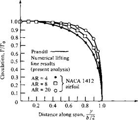
The procedure outlined above generally works smoothly and quickly on a high­speed digital computer. Typical results are shown in Figure 5.27, which shows the circulation distributions for rectangular wings with three different aspect ratios. The solid lines are from the classical calculations of Prandtl (Section 5.3), and the symbols are from the numerical method described above. Excellent agreement is obtained, thus verifying the integrity and accuracy of the numerical method. Also, Figure 5.27 should be studied as an example of typical circulation distributions over general finite wings, with Г reasonably high over the center section of the wing but rapidly dropping to zero at the tips.

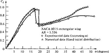
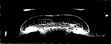
An example of the use of the numerical method for the nonlinear regime is shown in Figure 5.28. Here, Cl versus a is given for a rectangular wing up to an angle of attack of 50°—well beyond stall. The numerical results are compared with existing experimental data obtained at the University of Maryland (Reference 19). The numerical lifting-line solution at high angle of attack agrees with the experiment to within 20 percent, and much closer for many cases. Therefore, such solutions given reasonable preliminary engineering results for the high-angle-of-attack poststall region. However, it is wise not to stretch the applicability of lifting-line theory too far. At high angles of attack, the flow is highly three-dimensional. This is clearly seen in the surface oil pattern on a rectangular wing at high angle of attack shown in Figure

Figure 5.27 Lift distribution for a rectangular wing; comparison between Prandtl’s classical theory and the numerical lifting-line method of Reference 20.

Figure 5.28 Lift coefficient versus angle of attack; comparison between experimental and numerical results.

5.29. At high a, there is a strong spanwise flow, in combination with mushroom­shaped flow separation regions. Clearly, the basic assumptions of lifting-line theory, classical or numerical, cannot properly account for such three-dimensional flows.

For more details and results on the numerical lifting-line method, please see Reference 20.

Figure 5.29 Surface oil flow pattern on a stalled, finite rectangular wing with a Clark Y-14 airfoil section. AR = 3.5, a = 22.8°, Re = 245,000 (based on chord length). This pattern was established by coating the wing surface with pigmented mineral oil and inserting the model in a low-speed subsonic wind tunnel. In the photograph shown, flow is from top to bottom. Note the highly three-dimensional flow pattern. (Courte$y of Allen E. Winkelmann, University of Maryland.}