AN EXTENSION

In the above method, /ад2(Fu(P(juj), N(X, u))) is to be computed at each point (X, u>) of a gridding. The robustness margin r(X, u>) is then visualized as a function ofX and ы on a 3D plot (see section 5.). Nev­ertheless, a peak value of y&2(Fu(P(juj),N(X, uj))) may be missed with such a gridding (i. e. when this peak value lies between two points of the gridding), and the robustness properties of the closed loop would be overevaluated.

A simple method is proposed here for avoiding a gridding of the mag­nitude X, by treating this magnitude (more precisely the SIDF N(X, u>)) as an additional (fictitious) uncertainty. Frequency ш is fixed. An aug­mented skewed Ц problem is obtained. Even if the method is not applic­able to all kinds of nonlinearities, it can be applied to a large class of usual (especially memoryless) ones.

• The aim of this subsection is to compute the robustness margin r(o>)

r(ui) = min_ r(X, w) (12.24)

хє[£, X]

Lemma 3..5 provides an alternative definition of r(u>). The proof is trivial when using Proposition 3..3.

LEMMA 3..5 If:

l/r{u) < l/HA2(P22(ju)) _

2/ det(I – Pn(ju})N(X, u})) ф 0 for all X Є [X, X]

then:

-ГТ = max_ /j, A2{Fu{P(ju>),N{X, u>))) r(u) xe[x, x]

• Consider first a classical nonlinearity, namely a saturation у = Ф(ж)

у = x if x < 1 = +1 if X > 1

= -1 if X < -1 (12.26)

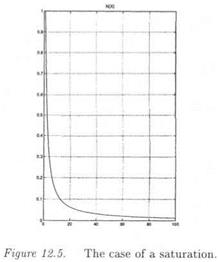
The associated SIDF N(X), which does not depend on frequency u> and which is a real scalar, can be computed as (see also Figure 12.5):

With respect to Figure 12.5 and equation (12.27), it is obvious that X € [0, oo] leads to N{X) Є [0, 1].

• Consider now the generic case of a memoryless SISO nonlinearity: here again, the SIDF N(X) is a real scalar which does not depend on frequency и). X Є [X, X] can thus be translated into N(X) Є [jV, N], The idea is thus to rewrite N(X) as:

N{X) = a0 + a xx (12.28)

where the oti s are chosen so that x — [ — 1 , 1 ] leads to N(X) є [N, IV].

• In the general case of a diagonal MIMO memoryless nonlinearity Ф = сІіад(Фі), the SIDF can be written as:

N(X) = Z0 + ZiA і (12.29)

where the Zi s are fixed diagonal matrices and Ді = diag(xi). X denotes now a vector of magnitudes Xu while_N(X) is a diagonal matrix. Here again, Ді Є D leads to N(X) e [N_, N], • Applying now equation (12.29) to Figure 12.3, this Figure can be trans­formed into Figure 12.4, where:

■ the fictitious real model perturbation — i contains the uncertainties Xi in the magnitude vector X, or equivalently in the SIDF N(X).

■ the real model perturbation Д2 contains the true parametric uncer­tainties.

■ Matrices Zi ’ s are incorporated in the transfer matrix P(s).

The following Proposition presents a method for computing r(u). PROPOSITION З..6 Let the interconnection structure of Figure 12.4. If:

1/г{ш) < 1/мд2(РЫ. Н)

2//W-PiiO’w)) < 1

then:

г’д(P(jw)) is the skewed s. s.v. associated to the complex matrix P(jaj) and to the real model perturbation Д = diag{Aі, Дг)- Ді is to be main­tained inside its unit hypercube D.

Remarks:

(i) The assumptions of this Proposition are essentially extensions of the assumptions in Proposition 3..3. Note especially that the second assump­tion in Proposition 3..6 means that the necessary condition of oscillation is not satisfied by the nominal closed loop system, for frequency to and for a vector of magnitudes X є [X, X].

(ii) A frequency gridding can be avoided, by treating ю as an additional uncertainty in an augmented ц problem (see section 3. of chapter 7).

(Hi) The above method can be applied to nonlinearities, which are not necessary memoryless: The SIDF N(X, uj) may depend on w and it may take complex values. For a fixed value of u>, the key point is to be able to reparameterize N(X, u>) in an affine way as N(X, u>) = ao + оцх, so that the trajectory of N(X, w) in the complex plane is the same when imposing s Z [ — 1 , 1 ] and X Є [X, hi­proof: this Proposition is an extension ofProposition 3..3 and Lemma 3..5 The issue is to compute the maximal value ofr(X, u>) over X Є [X, X]. The fictitious parametric uncertainties Xi associated to N(X) must con­sequently remain inside the unit hypercube D, while the true parametric uncertainties in Д2 are to be expanded, until the necessary condition of oscillation in equation (12.14) is satisfied.