Effect of Aspect Ratio

Returning to Equations (5.61) and (5.62), note that the induced drag coefficient for a finite wing with a general lift distribution is inversely proportional to the aspect ratio, as was discussed earlier in conjunction with the case of the elliptic lift distribution. Note that AR, which typically varies from 6 to 22 for standard subsonic airplanes

Figure 5.1 8 Induced drag factor S as a function of taper ratio. (Source: McCormick, B. W., Aerodynamics, Aeronautics, and Flight Mechanics, John Wiley & Sons, New York, 1979.)

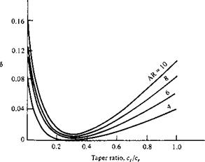
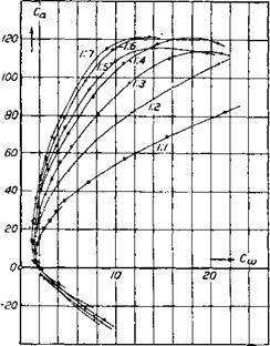
and sailplanes, has a much stronger effect on Cdj than the value of <5, which from Figure 5.18 varies only by about 10 percent over the practical range of taper ratio. Hence, the primary design factor for minimizing induced drag is not the closeness to an elliptical lift distribution, but rather, the ability to make the aspect ratio as large as possible. The determination that Cdj is inversely proportional to AR was one of the great victories of Prandtl’s lifting-line theory. In 1915, Prandtl verified this result with a series of classic experiments wherein the lift and drag of seven rectangular wings with different aspect ratios were measured. The data are given in Figure 5.19. Recall from Equation (5.4), that the total drag of a finite wing is given by

C2

^L

neAR.

The parabolic variation of CD with CL as expressed in Equation (5.63) is reflected in the data of Figure 5.19. If we consider two wings with different aspect ratios ARi and AR2, Equation (5.63) gives the drag coefficients CDд and C0,2 for the two wings as

Assume that the wings are at the same Cl. Also, since the airfoil section is the same for both wings, Cd is essentially the same. Moreover, the variation of e between the

Figure 5.1 9 Prandtl’s classic rectangular wing data for seven different aspect ratios from 1 to 7; variation of lift coefficient versus drag coefficient. For historical interest, we reproduce here Prandtl’s actual graphs. Note that, in his nomenclature, Ca = lift coefficient and Cw = drag coefficient. Also, the numbers on both the ordinate and abscissa are 100 times the actual values of the coefficients. (Source: Prandtl, L., "Applications of Modern Hydrodynamics to Aeronautics," NACA Report No. 116, 1921.)

wings is only a few percent and can be ignored. Hence, subtracting Equation (5.64b) from (5.64a), we obtain

Equation (5.65) can be used to scale the data of a wing with aspect ratio AR2 to correspond to the case of another aspect ratio AR|. For example, Prandtl scaled the data of Figure 5.19 to correspond to a wing with an aspect ratio of 5. For this case,

Equation (5.65) becomes

Сд, і = Co,2 H———– f – — —c—^ [5.66]

же 5 AR2/

Inserting the respective values of Cd,2 and AR2 from Figure 5.19 into Equation (5.66), Prandtl found that the resulting data for Сд, ь versus Cl collapsed to essentially the same curve, as shown in Figure 5.20. Hence, the inverse dependence of Cd, і on AR was substantially verified as early as 1915.

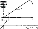
There are two primary differences between airfoil and finite-wing properties. We have discussed one difference, namely, a finite wing generates induced drag. However, a second major difference appears in the lift slope. In Figure 4.4, the lift slope for an airfoil was defined as a0 = dci/da. Let us denote the lift slope for a finite wing as a = dCL/da. When the lift slope of a finite wing is compared with that of its airfoil section, we find that a < a0- To see this more clearly, return to Figure 5.4, which illustrates the influence of downwash on the flow over a local airfoil section of a finite wing. Note that although the geometric angle of attack of the finite wing is a, the airfoil section effectively senses a smaller angle of attack, namely, aetf, where acff = a — a,-. For the time being, consider an elliptic wing with no twist; hence, a, and acff are both constant along the span. Moreover, q is also constant along the span, and therefore CL = ci. Assume that we plot Cl for the finite wing versus aeff, as shown at the top of Figure 5.21. Because we are using аеп the lift slope corresponds

Figure 5.30 Data of Figure 5.19 scaled by Prandtl to an aspect ratio of 5.

to that for an infinite wing ao. However, in real life, our naked eyes cannot see aeff; instead, what we actually observe is a finite wing with a certain angle between the chord line and the relative wind; that is, in practice, we always observe the geometric angle of attack a. Hence, CL for a finite wing is generally given as a function of a, as sketched at the bottom of Figure 5.21. Since a > aeff, the bottom abscissa is stretched, and hence the bottom lift curve is less inclined; it has a slope equal to a, and Figure 5.21 clearly shows that a < a(). The effect of a finite wing is to reduce the lift slope. Also, recall that at zero lift, there are no induced effects; i. e., a, = CDJ = 0. Thus, when Cl = 0, a = aeff. As a result, a/ =0 is the same for the finite and the infinite wings, as shown in Figure 5.21.

The values of a о and a are related as follows. From the top of Figure 5.21,

dCL

d(a — ctj)

Integrating, we find

CL = ao(a — at) + const

Substituting Equation (5.42) into (5.67), we obtain

[5.68]

Lift curves for an infinite wing versus a finite elliptic wing.

Differentiating Equation (5.68) with respect to a, and solving for dCi/da, we obtain

dCb _ _ do

da 1 + qq/^AR

Equation (5.69) gives the desired relation between a0 and a for an elliptic finite wing. For a finite wing of general planform, Equation (5.69) is slightly modified, as given below:

1 + (a0/7rAR)(l + r)

In Equation (5.70), г is a function of the Fourier coefficients A„. Values of r were first calculated by Glauert in the early 1920s and were published in Reference 18, which should be consulted for more details. Values of r typically range between 0.05 and 0.25.

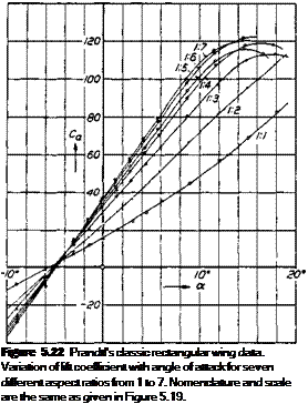
Of most importance in Equations (5.69) and (5.70) is the aspect-ratio variation. Note that for low-AR wings, a substantial difference can exist between a0 and a. However, as AR oo, a ao – The effect of aspect ratio on the lift curve is dramat­ically shown in Figure 5.22, which gives classic data obtained on rectangular wings byPrandtlin 1915. Note the reduction in dCi/da as AR is reduced. Moreover, using the equations obtained above, Prandtl scaled the data in Figure 5.22 to correspond to an aspect ratio of 5; his results collapsed to essentially the same curve, as shown in

Figure 5.23. In this manner, the aspect-ratio variation given in Equations (5.69) and (5.70) was confirmed as early as the year 1915.