Adaptive Sparse Grid for High-Dimensional Integration
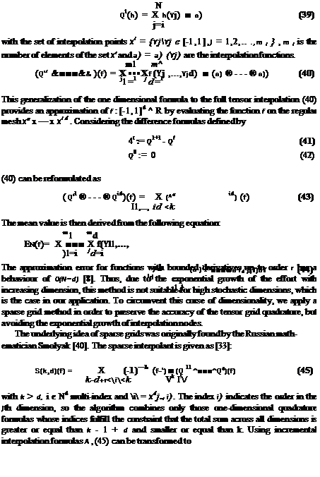
The mean value of the robust optimization problem depending on the current design vector is required in each iteration of the optimization algorithm. Since we cannot solve this integral analytically, we have to approximate it in appropriate, efficient way. Several possibilities can be found in the literature, the most common are: Monte-Carlo simulation, respectively general sampling methods, full tensor grid interpolation and sparse grid interpolation. Their efficiency depends on the dimension d of the probability space Qd and on the properties of the integrand f (y, p, yd). Each of these methods provides an approximation En of the mean value E( f) by evaluating the function f (y, p, yd) in N integration points yj, •••, Wn and summing the results f (yi, p, yld) multiplied with the weights 03, •••, (0N up
N
En = ^Юі • f (yi, p, yd) (38)
i=l
The sampling methods randomly select realizations of the uncertainties in the given probability space and take some kind of average of the function values at these points which converges to the exact value of the integral due to the law of large numbers. The advantage of this approach consists of the straightforward implementation, the algorithm only needs the underlying integration space as input and function evaluations at the randomly selected points. But on the other hand, the expected convergence rate 0(N~2) requires a large number of function evaluations to ensure a given error tolerance. In our application, one function evaluation is very expensive since the solution of the flow equation, Euler or Navier Stokes equation, is needed. So, the sampling methods, even the improved methods which use additional information in order to select the realizations, are not an appropriate choice in our case to compute the mean value in our optimization problem.
Another possibility obtaining the objective value is the full tensor grid quadrature derived from the full tensor product of the one-dimensional interpolation formulas. Constructing the multi-dimensional interpolation, we first consider the following one-dimensional interpolation formula in order to approximate a function h : [—l, l] ^ R:

5(k, d)(f) = X A1 (f)
i<k
= S(k – 1,d)(f) + X A1 ®—®Ad) (f)
i=k
with A = Ql+l – Ql, Q° = 0 and S(d – 1, d) = 0. The collection of all the interpolation points ( )
H (k, d) = У (X11 x—xX‘d) (46)
k—d+1<i<k
is called a sparse grid of level k.
The derivation of the sparse grid suggests the use of nested interpolation functions due to the recursive construction. In the literature, the most popular choice of the collocation points is the Clenshaw-Curtis grid at the non-equidistant extrema of the Chebyshev polynomials and the underlying interpolation formula is the Chebyshev-Gauss-Lobatto formula.


