AN APPLICATION

The necessary condition of oscillation is used to synthesize a controller, which modifies the characteristics (magnitude and frequency) of a limit – cycle. This is an interesting engineering problem, since a limit-cycle is not necessarily a trouble in a nonlinear closed loop: a high frequency limit-cycle can linearize in an approximate way the nonlinear closed loop. Within the fj, framework, the following example illustrates that a troublesome limit-cycle (with a large magnitude and a low frequency) can be moved into a suitable limit-cycle (with a smaller magnitude and a higher frequency). For the sake of clarity, this example is chosen will­ingly simple: it is nevertheless straightforward to extend the method to the more general case of a MIMO nonlinearity, with a more complex parameterization of the controller.

Let the closed loop system of Figure 12.9, where G(s) is the plant model and K(s) the controller:

1

s2 + 1.4s + 1
К

агв2 + ais + 1

with К = 20, а,2 = 1/ta2 = 0.01, a = 2£/u; = 0.14, w £ = 0.7.

A saturation is present at the plant input (see equation (12.26)). A limit-cycle is obtained, whose predicted characteristics are a magnitude X = 2.46 and a frequency ш — 3.16 rad/s (using the method of subsec­tion 2.1). The characteristics obtained in simulation are X = 2.56 and и = 3.08 rad/s: these values are thus very close to the predicted ones, which means that the first harmonic assumption is valid. The limit-cycle is moreover stable.

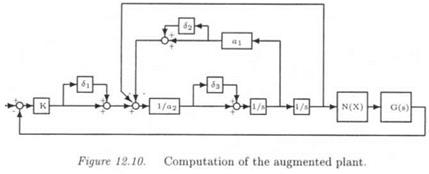
This limit-cycle is to be moved by retuning the controller K(s). The tuning parameters are K, ai and a 2 (more precisely 1 / аг). The aug­mented plant of Figure 12.3 is simply obtained by directly introducing "uncertainties" Si into the physical model of K(s) (see Figure 12.10 – N(X) is the SIDF of the saturation). The real model perturbation Д2 is Д2 = diag(6i, 62,63).

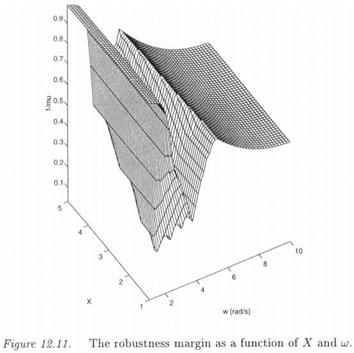
The quantity l/max(^a(Fu(P(jw), AT(Jf, w))),^2(P220’w))) is presen­ted as a function ofX and ш on Figure 12.11 (see Corollary 3..4) [15]. Re­member that there is a limit-cycle in the nominal closed loop system, at

X = 2.46 and w = 3.16 rad/s. As a consequence, r(X, ш) = Oat this point, and r(X, u) increases around this critical point.

The limit-cycle is to be moved at X = 1.2 and ш = 6.2 rad/s (i. e. the frequency of the limit-cycle is roughly multiplied by a factor 2, while the magnitude is divided by the same factor). А ц lower bound is computed for fj, A2(Fu(P(ju}),N(X))) at this new point (X, w), namely 1.22. An associated model perturbation A?; is provided as:

<5i = 0.6906 S2 = -0.7893 S3 = 0.8203 (12.38)

This model perturbation is applied to K(s), which becomes:

33.81

0.0055s2 + 0.0295s + 1

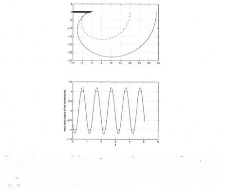
Here again, a stable limit-cycle is obtained in simulation, with A = 1.207 and ш = 6.282 rad/s (see Figure 12.12).

Remark: remember first that r(X, ui) represents the minimal size of the model perturbation Д 2 , for which a limit-cycle is obtained at [Х, ш) (see definition 3..2). In the context of the above design problem, a limit-cycle is obtained for the nominal value of the controller, and this controller is retuned in order to move the limit-cycle at a point (X, u>): it is thus interesting to use the minimal size model perturbation associated to r(X, w). Indeed, the corresponding controller can be considered as the controller, which is the closest to the nominal one, and which moves the limit-cycle at (X, ci).

— 1 /N(X) in the Nyquist plane, while the lower subfigure represents the input and output of the nonlinearity (when the limit-cycle is obtained) – the dashed plot on the top Figure represents K(ju)G{jui) for the initial value of the controller, whereas the solid line represents K(ju>)G(jui) for its final value.

4. CONCLUSION

The general aim of this chapter was to check the existence or the ab­sence of limit-cycles in a closed loop subject to parametric uncertainties. The aim was more precisely to show that this nonlinear problem can be solved with existing tools of linear robustness analysis (i. e. analysis of

the robustness properties of an LTI closed loop system, subject to LTI

model uncertainties):

■ Computation of the frequency response of a parametrically uncertain transfer function (Kheel and Bhattacharyya, 1994).

■ Use of the LFT framework to transform the original problem into an equivalent standard interconnection structure.

■ Computation of upper and lower bounds of the (skewed) structured singular value.

This page intentionally left blank