Euler Flow

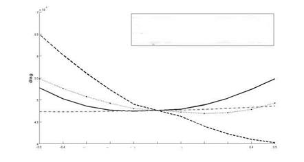
As Fig. 10 shows, the third eigenvector has no impact on the objective function, hence it can be rejected from the Karhunen-Loeve basis and the dimension of the integral is reduced. This behaviour is also reflected by the introduced indicator. Consequently, the mean value is given by

e(/ (y, P, yreduced (x, Z))) =

—— 1. eigenvector	indicator:	2.255806Є-04
—– 2. eigenvector	indicator:	-1.421137e-03
— 3. eigenvector	indicator:	7.722186Є-06
■■"•■■■4. eigenvector	indicator:	-4.745173Є-04

-0.3 -0.2 -0.1 0 0.1 0.2 0.3

perturbations

Fig. 10 Drag performance of the first four eigenvectors on the target functional

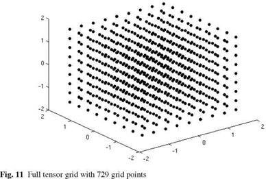
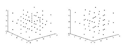
If one approximate the expected value (75) using a full tensor grid interpolation (40), 729 grid points will be needed to reach the error tolerance of 3 • 10_4. The resulting full grid is shown in Fig. 11. Since we want to compare the efficiency of the different introduced methods, we have chosen multilinear hierarchical basis function as ansatzfunctions for the sparse and full tensor grid. The sparse grid method can reduce the computational effort by a factor of 10 maintaining the same approximation quality. The corresponding grid is depicted in Fig. 12. As Fig. 12

Fig. 12 Sparse grid with 69 grid points and locally refined sparse grid with 52 grid points

shows, the number of grid points can again be reduced from 69 grid points to 52 grid points, i. e. a reduction of 17 flow simulations in each iteration is reached us­ing a local refinement strategy. Since the optimization requires the evaluation of the mean value in each iteration, this reduction by factor 15 compared with the full grid takes place in each step of the optimization algorithm and hence significantly speed up the whole algorithm. The construction of the adaptive sparse grid although needs some additional function evaluations in order to compute the adaptivity indicator, but this amount of computational effort occurs outside the optimization loop, i. e. these costs are negligible.

Beside the local refinement strategy, a dimension adaptive sparse grid was in­troduced in section 5.1. The main advantage of this approach lies in the possibility to choose the underlying quadrature formulas problem dependent. As discussed be­fore, Gaufi-Hermite formulas are used. Due to the higher accuracy of Gaufi-Hermite

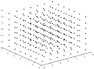
Fig. 13 Full tensor grid with 343 grid points

Fig. 14 Sparse grid with 37 grid points and dimension adaptive sparse grid with 21 grid points

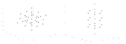
quadrature formulas, an error tolerance of 10~5 is required. An usual sparse grid can reduce the number of grid points from 343 to 37, again almost a factor of 10. The dimension adaptive strategy results in a grid with 21 points (cf. Fig. 14). The comparison of the two refinement strategies shows that the use of problem dependent quadrature formulas can significantly reduce the size of the grid and in­crease the approximation quality at the same time. Hence, the objective function in the semi-infinite formulation is approximated by the dimension adaptive grid with 21 grid points. the next two Fig. 15,16 compare the results of the robust optimization and of the single setpoint optimization, i. e. without considering any uncertainties

‘ 0 2 4 6 8 10 12

Fig. 16 Lift performance of the 21 perturbed geometries

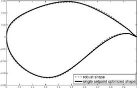The drag and lift performance is plotted against the 21 perturbed geometries and the dashed line in Fig. 15 indicates the mean value of the drag. The robust optim­ization improves the mean value of the target functional and also leads at the same time to a better lift performance over the whole range of perturbations, whereas the single setpoint optimization is infeasible in more than the half of the considered grid points. Summing it all up, it can be said that the robust optimization leads to a better lift to drag ratio than the single setpoint optimization and the resulting profile is more robust against small perturbations of the shape itself. Last, we will compare the different resulting shape in Fig. 17.

Although we have assumed only small perturbations of the shape itself (cf. Fig. 7), the difference between the robust shape and the single setpoint is well recognizable.