Enforcing Wall Boundary Conditions on Curved Surfaces

When curved surfaces are involved in a computation, very often a body-fitted grid is used. It will now be assumed that the computation grid is on a set of orthogonal

Figure 6.17. Orthogonal curvilinear co­ordinates (f, n, Z) forming a body-fitted curved surface.

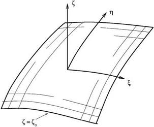curvilinear coordinates f (x, y, z), n(x, y, z), and Z (x, y, z). The coordinate system is orthogonal, meaning that

Vf ■ Vn = Vn ■ VZ = VZ ■ Vf = 0. (6.26)

Without the loss of generality, the curved boundary surface is taken to be on the Z = Zo coordinate surface as shown in Figure 6.17. The normal to the surface is in the direction of VZ.

The Euler equation in curvilinear coordinates (f, n, Z) is given by Eq. (5.61).Let U = v ■ Vf, V = v ■ Vn, W = v ■ VZ (the contravariant velocity components), i. e.,

n 9f 9f 9f

dx 9y 9 z

9n 9n 9n

V = u + v + w dx dy 9 z

w 9Z 9Z 9Z

W = u + v + w . dx dy 9 z

The momentum equation in the Z direction may be found by multiplying the second equation of (5.61) by Zx, the third equation by Zy, and the fourth equation by Zz (subscript denotes partial derivatives), then summing up the three equations. On being written out in full, the equation is as follows:

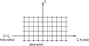
For inviscid flow, the wall boundary condition is W = 0on Z = Zo (the solid surface). To enforce the wall boundary condition, it is recommended to include a set of ghost points on the surface Z = Zo – AZ as shown in Figure 6.18. At each ghost point, a ghost value of p is included in the computation. The computation is carried out in the (f, n, Z) space. It is similar to computation in a Cartesian coordinate system.

Figure 6.18. Computational grid and ghost points near a solid wall in a com­putational domain.

For all mesh points inside the computation domain, the discretized form of Eq. (5.61) is used. For all flow variables, with the exception of p, backward difference stencils for d/dz are implemented for points in the boundary region. This is to keep the stencil points inside the computational domain. For 9p/dz, the stencils are extended to the ghost points. For mesh points lying on the solid surface z = Zo, instead of the second, third, and fourth equation of (5.61), Eq. (6.28) and two of the three equations are used. Let (l, m, n) be the spatial indices in the Z, n, and z directions, respectively, and z = zo corresponds to n = N, the discretized form of Eq. (6.28) at n = N, taking into account that the boundary condition W = 0 at z = zo, is as follows:

where superscript k is the time level.

The ghost value of pressure, pf}m N—1, may now be calculated by Eq. (6.29). The explicit formula is as follows:

p(k) =__ 1 a51 „0

pl, m,N—1 = a51 U1 pl

a—1 j=0

With the ghost value of p found, the computation can proceed as in the case of a flat wall.

For viscous flows, the full Navier-Stokes equation must be used in the computa­tion. The boundary conditions on the curved solid surface are the no-slip conditions. Because the stress terms are fairly complicated in curvilinear coordinates, the use of ghost values of shear stresses to enforce the no-slip boundary conditions would require a good deal of effort. A less complicated approach is to set (u, v, w) to zero on z = Z0 (n = N). To avoid the computation becoming an overdetermined system, the three momentum equations will not be used for mesh points right at the solid surface. For density p and pressure p on the solid surface, they are to be computed by means of the continuity and energy equations. Although this approach is a bit less accurate, this way of treating the curved wall boundary condition has been found to be quite efficient, easy to implement, and offers reasonably accurate results.

EXERCISES

6.1. Consider solving the one-dimensional wave equation

d 2U 2d2U

dt2 C dx2

in a finite domain. The equation has two solutions:

u = F(x – ct) + G(x + ct),

where F and G are arbitrary functions. The solution F (x – ct) represents a wave propagating to the right, and the solution G(x + ct) represents a wave propagating to the left.

Develop a radiation boundary condition for the right and the left boundary of the computation domain.

6.2. For problems with spherical symmetry, it is advantageous to use spherical coor­dinates (R, в, ф). The linearized Euler equations in spherical coordinates for prob­lems with spherical symmetry are (9/9в = 0, Э/Эф = 0) as follows:

— + 1 dp = 0

91 p0 d R

where «0 = yp0/p0. The general solution of (3) is

_ F(R – a0t) + G(R + a0t)

P _ R + R ‘ ()

F and G are arbitrary functions. Derive a radiation boundary condition for p at large R. In solving the system of equations (1) and (2) a boundary condition for v is also needed. Derive a boundary condition for v.

6.3. Use dimensionless variables with respect to the following scales:

Ax _

aO (ambient sound speed) _ Ax

a

pO _ density scale
P^aO _ pressure scale

The linearized two-dimensional Euler equations on a uniform mean flow are to be solved

9 U 9 E 9 F

dt dx 9y

where

P		Mx P + u		My P + v
u	, E _	Mxu + p	, F _	Myu
v		Mxv		MyV + p
p		Mxp + u		Myp+v

Mx and My are constant mean flow Mach number in the x and y directions, respec­tively. Use a computation domain -100 < x < 100, -100 < y < 100 embedded in free space.

(a) Let Mx = 0.5, My = 0. Solve the initial value problem, t = 0.

– <ln2>(^У

■- (ln2> (Цгу + 0.1 exp [- (ln2><K^6^У

Note: The mean flow is in the direction of the diagonal of the computational domain. Compute the distributions of p, p, and u at t = 60, 80, 100, 200, and 600.

6.4. The exact solution of the initial value problem of the diffusion equation,

d u f 9 2u 9 2uл

9t 9 x2 + 9 y2,

(x2+y2 >

-(ln2> b-

Suppose one is interested to find the solution computationally by using the DRP scheme. Let Ax = Ay be the length scale and (Ax)2/к be the time scale, so that the nondimensional diffusion equation becomes

du d2U d 2U

dt dx2 dy2

t = 0

To solve this problem computationally in a finite domain requires numerical bound­ary conditions. For diffusion equations, the asymptotic solution is not useful for constructing a numerical boundary condition.

It is observed, because of the diffusive nature of the solution, that the solution at a point depends mainly on the solution on the side closer to the source. For this reason, it is recommended that one use backward difference stencils at mesh points close to the exterior boundaries of the computation domain. No other spe­cific boundary conditions at the outer boundaries of the computation domain is needed.

Compute the solution on a 100 x 100 mesh with b = 3. Compare your numerical solution with the exact solution by plotting u(x, 0, t) at t = 20, 40, 80,160, 300. See Appendix D for helpful suggestions.

6.5.

Consider one-dimensional flow and acoustics in a nozzle attached to a long duct of uniform cross section as shown. For calculating the flow and acoustic waves in the nozzle, it is decided to use a computation domain encompassing the variable area part of the nozzle. The right boundary of the computation domain is in the uniform duct. A small-amplitude sound wave of angular frequency ы propagates from the uniform duct into the nozzle region. Part of this wave is transmitted through the nozzle throat and a part of it is reflected back into the uniform duct.

Let u, p, and p be the mean flow in the uniform area duct. The linearized gov­erning equations in the duct are the continuity, momentum, and energy equations.

9p _du _9p dt H 9x 9x	(1)
d u 9 u 1 9 p —– + u—– 1——- = 0 dt dx p dx	(2)
d p _9 p _____ 9 u n dt dx 1 dx	(3)

The upstream propagating acoustic wave in the uniform duct is given by

(4)

where a = (yp/p)1/2 is the sound speed. F is a known function.

Develop a set of outflow boundary conditions for use on the right side of the computation domain.

If the left side of the nozzle is attached to another long uniform duct, hot spots in the form of entropy waves are convected downstream by the mean flow into the nozzle. The entropy wave solution may be written as

p		1
u	=	0
p		0

H(x — Ut),

where U is the local mean flow velocity of the uniform duct and H is a known function characterizing the density (temperature) distribution.

Develop a set of inflow boundary conditions for use on the left side of the computation domain.

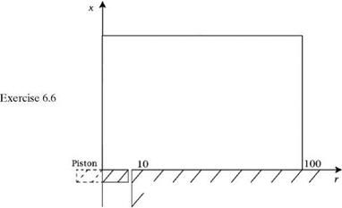
6.6. Consider acoustic radiation from an oscillating circular piston in a wall as shown below.

Let the radius of piston be R and the velocity of piston be u = є sin(nt/5). Use a computational domain 0 < x < 100, 0 < r < 100. The wall and the piston are at x = 0. The cylindrical coordinate system is centered at the center of the piston. With axisymmetry, the dimensionless linearized Euler equation is

p		v		v r		u
u	9	0		0	9	p
			+
v	9 r	p	0	9 x	0
p		v		v r		u

= 0.

The initial conditions are

t = 0, p = u = v = p = 0.

Compute the time harmonic pressure distribution at the beginning, 1 /4,1 /2, and 3/4 of a period of piston oscillation.

Let e = 10 4, R = 10, ю = n/5. The exact solutions is

TO

6.7. A spherically symmetric acoustic pulse is initiated at time t = 0 by a small – amplitude pressure pulse of the following form:

p = p = ee – (ln2)[(x2+y2+z2 )/b2]

in a static environment. Here, the length scale is Ax = Ay = Az, the velocity scale is a0 (the speed of sound), the time scale is Ax/a0, the density scale is p0 (the mean gas density), and the pressure scale is p0a0. Compute the solution by solving the three­dimensional Euler equations in Cartesian coordinates. Take e = 10-4 and b = 3.

Let R = (x2 + y2 + z2)1/2 be the radial distance. The exact linearized solution is

p = e R – 1 e-(ln2)[(R-t)/b]2 + R + 1 e-(ln2)[(R+t)/b]2

p 2R 2R

Note: A computer code for this problem is provided in Appendix G.