Parabolic Drag Polar

Modeling aerodynamic forces and moments of aerospace vehicles can be a formidable task. Multimillion-dollar wind-tunnel facilities have been built and supercomputers put to work to measure, calculate, and predict the flow phenomena. A mathematical framework must be found to express these data in a form that can be programmed for the computer. In Chapters 9 and 10 you will encounter models for missiles and aircraft at increasing levels of sophistication. For three- DoF simulations, we can confine ourselves to expressions that relate drag and lift by simple polynomials.

We go back to the latter part of the 19th century and find Otto Lilienthal exper­imenting with hang gliders. He took his hobby very seriously and is credited with relating lift and drag by what he called “die Flugpolare” (the drag polar). After his accidental death in 1896, the Wright brothers6 credited him in 1901 with laying the foundation of flight by experimentation.

The lift force L is normal to the velocity vector of the aircraft wrt the air and is contained in the plane of symmetry of the aircraft. The drag force D is parallel and in the opposite direction of the velocity vector. Nondimensional aerodynamic coefficients are formed from the dynamic pressure q and the reference area S (airplanes use wing area and missiles employ body cross section).

Lift coefficient:

Drag coefficient:

with q = (p/2)V2, p the air density, and V the speed of the aircraft relative to air. Both coefficients are assumed to be functions of the following parameters:

Cl, Cd = /{Mach, angle of attack, power on/off, shape}

Mach number, the ratio of vehicle velocity over sonic speed, can have a signifi­cant effect on the coefficients during the transonic and supersonic flight regimes. The main effector however is the angle of attack, which, with only small varia­tions, changes the lift coefficient decisively. Depending on the installation of the propulsion unit, the airflow around the wing or tail modifies the drag character­istics. Particularly for missiles with boost motors, the drag increases significantly during the coast phase. Naturally, the shape of the vehicle determines the overall aerodynamic performance, but the size of the vehicle has only a minor influence on the coefficients. This insensitivity to scale justifies much of the considerable wind-tunnel investments.

When drag data are plotted against lift, a near parabolic curve emerges for any given Mach number. What a break for the aerodynamicist! He can model the func­tional relationship by a second-order polynomial, called the parabolic drag polar.

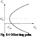
CD = CDo+k(CL-CL()2 (8.18)

The parabola is shown in Fig. 8.4. Not surprisingly, drag is never zero even at zero lift. It has a minimum value of Co0, which may occur at a nonzero lift value C/ o. A parabolic drag polar thus shifted upward is called an offset polar. The factor к determines the drag increase caused by deviation from minimum drag and is referred to as the induced drag coefficient.

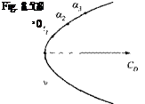
If the minimum drag occurs at zero lift, the function simplifies to a centered polar (see Fig. 8.5):

The drag polar is centered on the drag axis if the vehicle has two planes of symmetry—like a conventional missile—or if a wing with symmetrical airfoil is the dominant lifting surface. The parameter of the parabola is the angle of attack a. The higher the angle of attack is, the greater the lift and drag forces, up to the point when the flow starts to separate from the main lifting surface. Thereafter, lift breaks down, but drag keeps increasing, and the parabolic model has lost its usefulness.

The noninduced drag coefficient Сд> models such phenomena as surface fric­tion, profile drag, and supersonic wave drag. The second term represents the in­duced drag caused by lift. For vehicles that traverse through more than one Mach region—subsonic, transonic, supersonic, or hypersonic—the coefficients CDo, Cl0, Ci, к must be modeled as functions of Mach number.

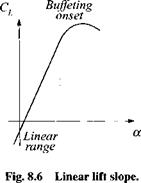
The drag polar presupposes that lift is given and drag is derived. In simulations, however, one prefers to specify the angle of attack as input rather than lift. A relationship must therefore be established between the lift coefficient and angle of attack. Fortunately, experimental evidence points to a linear relationship (see Fig. 8.6):

Cl = CLm + Ciaa

That linearity extends to the onset of flow separation, when lift brakes down rapidly. It is present over all Mach regimes. For vehicles with a centered drag polar, the lift slope goes through the origin, i. e., CiM = 0.

The parabolic drag polar is an aerodynamic model suitable for simple point – mass three-DoF simulations from subsonic to hypersonic flight regimes. Be careful,

however, and do not expect too much accuracy from the results. Imposing a second – order polynomial curve washes out minimum drag cups near the cruise conditions and, as already noted, does not account for the onset of buffeting. A parabola also assumes lift symmetry for positive and negative angles of attack—hardly the case for airplane wings with high-lift airfoils. Furthermore, we also neglected Reynolds-number dependency and skin-friction changes with altitude.

All of these shortcuts were taken to get you started with simple simulations. As you gather more data, you can abandon the parabolic fit in favor of higher-order polynomials or use tables to accurately model the functional relationship between the lift and drag coefficients. However, there are inherent restrictions that come with the point-mass approach.

One supposition is the neglect of the control surface effects on lift and drag. Their contribution could be included as so-called trimmed values, if we had a full force and moment model available for data reduction. However, in that fortunate case we may as well build a full six-DoF simulation.

Another assumption restricts the lateral maneuver to coordinated turns only, i. e., the aircraft banks without sideslipping. The same limitation applies to missiles, unless they possess rotational symmetry, in which case the lift and drag forces always lie in the load factor plane, irrespective of the body bank attitude. In effect, for both missiles and aircraft the drag polar applies to the aerodynamic forces in the load factor plane.

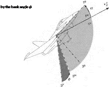
Figure 8.7 helps us to define the load factor plane. It coincides with the Is, 3s symmetry plane of the aircraft and contains the velocity vector v f of the aircraft wrt to Earth. The bank angle ф establishes the orientation of the load factor plane relative to the vertical plane, which contains the lv,3V axes (Iv coincides with vf). The angle of attack a positions the aircraft centerline above the velocity vector in the load factor plane. It is useful to introduce the load factor coordinate system. Its Iм axis is parallel and in the direction of the velocity vector vf and Iм coincides with 2s. In load factor coordinates the resultant aerodynamic force possesses lift and drag as its two components:

[fa]M=qS[-CD 0 – CJ (8.21)

The transformation matrix of the load factor wrt velocity coordinates is determined
and the aerodynamic force in velocity coordinates is therefore

[.faY = [? ]MV[fa]M = qS

As expected, the drag force opposes the aircraft velocity directly, and the lift force, modulated by bank angle ф, generates the horizontal maneuver force С/ sin ф and the vertical force —Ci cos ф.

Modeling the aerodynamics of airplanes and missiles with a parabolic drag polar is a quick way to get preliminary performance estimates of new concepts when the database is still scant. Furthermore, this simple approach is also quite useful for mission-level simulations with their frugal trajectory models. There, the aircraft and missiles are well defined; but because of the large number of participating vehicles, their fly-out simulations must be kept artless.

So far, we have dealt with the gravitational and aerodynamic forces. To complete the right-hand side of Newton’s law, we must address the force that overcomes gravity and drag, namely thrust. I shall discuss rocket and airbreathing propulsion in a form not just suitable for three-DoF models, but also quite applicable to five – and six-DoF simulations.