Applications

The applications draw on the two CADAC simulations CRUISE5 and SRAAM6, the cruise missile and the short-range air-to-air missile. We will analyze the output

E 0) о 3

Fig. 10.52 Medium roughness terrain, 30 Monte Carlo runs, mean and standard deviation.

using univariate and bivariate stochastic models. Of particular interest is the mod­eling of stochastic terrain, INS position error growth, impact accuracy, and launch envelopes. I will present only selected results; you can find more test cases on the CADAC CD.

In Sec. 9.3.3 I briefly described the random terrain, which models smooth, medium, and rough topography. A second-order power spectral density function is sampled for laying down the terrain ahead of the missile. Figure 10.52 shows the traces of 30 Monte Carlo runs and their univariate analysis, initiated at 3 s into flight. The mean altitude was set at 100 m. The mean of the stochastic traces deviates only slightly from this value. For an infinite number of runs, they would coincide. The spread of the tracks is characterized by the one-sigma band of ± 15 m. In CADAC the Monte Carlo technique is automated, and the univariate analysis is carried out by the utility program MCAP. EXE.

Another interesting study is the propagation of the INS position errors. In Sec. 10.2.4 I derived the error equations for space and terrestrial stabilized INS. Again making use of the CRUISE5 simulation with its terrestrial INS, Fig. 10.53 shows the 30 Monte Carlo replications before and after the start of the GPS up­dates. At launch the mean is slightly biased, and the one-sigma band is ±5 m. Starting with the first GPS update at 8 s into flight, the bias is eliminated and the stochastic error reduces to 1 m.

Bivariate distributions are usually related to miss calculations. They arise at aircraft landings, spacecraft docking, and missile intercepts. I use an air-to-air missile to illustrate the application.

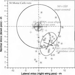
If you have solved Problem 4.11, you worked with the intercept plane that is used to record miss distance. Refer to the figure of Problem 4.11 to orient yourself. Fifty Monte Carlo shots were taken and recorded on the intercept plane in

Fig. 10.53 INS position error (north component) before and after GPS update, mean and standard deviation.

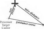
Fig. 10.54. The target aimpoint is centered at zero. As the right schematic indicates, miss distance is the vectorial sum of navigation and guidance errors. The crosses mark the point where the onboard processor places the target, and the stars are the actual impact points. On the intercept plane, the crosses cluster around the target, indicating that the navigation error is unbiased and equally distributed in both directions. Its 50% error ellipse is near circular. The impact points however are skewed by the 7-m bias and the 2:1 elliptical distribution. You as analyst will be asked the question whether the miss distance can be represented by the univariate CEP. How would you answer? The CEP is drawn, centered on the target, with a radius of 8 m. Is it an accurate measure of miss? I recommend that you give your customer the complete picture, explain the difference between univariate and bivariate distributions, and let him, according to his needs, make that judgement. The CADAC utility program KPLOT/BIVAR will help you prepare your presentation.

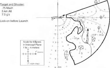
Figure 10.54 is based on a single engagement geometry between launch and target aircraft. It does not portray the performance of the missile under all possible launch conditions. The launch envelope of Fig. 10.55 provides that total picture. The scenario is a close-in engagement with both aircraft maneuvering at 7.5 g. The shooter (launch aircraft) is at the center of the envelope, whereas the target aircraft can be located anywhere, but maneuvering such that both canopies face each other. As long as the target is within the outer contour (at missile launch) it will be intercepted with the CEP indicated by the inner contours. To provide also the bivariate distributions, at selected points the bias and 50% miss ellipse are drawn at a magnified scale, as indicated in the box. For example, pick point 4 as the location of the target aircraft at missile launch. At intercept the CEP is less than 10 m with a bias of 8 m and an elliptical distribution about the mean as

large! Center

U’mile Impact

Fig. 10.55 Launch envelope, shooter centered.

shown. Surveying the whole envelope, you see how bias and miss ellipse change with the engagement geometry.

Figure 10.55 packs a multitude of information into one graph. It can only be generated in reasonable time if the whole process is automated. The CADAC SWEEP methodology provides the wherewithal. You set up a Monte Carlo sweep run and let your computer chew on it over night. The next morning, you execute the SWEEP utility program with the IMPACT. ASC file from the previous night and produce a graph similar to my example. Your customer will be duly impressed.

Enough said of the elements of six-DoF simulations! I covered a smorgasbord of specialties, which, combined with the information of Chapters 8 and 9, should give you a broad taste of the variety of subsystems. Other specialties that I did not serve up you will have to find in the references. Unfortunately, much of the information lingers in unpublished notebooks of specialists. To round out this chapter, I will briefly describe three typical six-DoF simulations.