Univariate Gaussian distribution

The simplest case is the one­dimensional output. Because we can assume the output parameters to be Gaussian distributed, our model is the univariate density function of the random variable x with mean цх and standard deviation ox:

1 (t-Д.;)2

p(x) =——- -=e (10.126)

Gx’Vl’K

To calculate the mean ix and standard deviation ox from the output ensemble of your MC runs X], X2,…. x,-….. xn, you can use the following equation:

With these values the density function p(x) is determined, but it lacks intuitive­ness. If we integrate over the function, we get an easier-to-understand probability statement of the random variable x, namely, that the probability that x assumes the values between a and b equals the area under the density function:

P(a < x < b) = ( p(x)dx (10.128)

J a

You have heard of the so-called one-sigma, two-sigma, and three-sigma accuracy statements. For instance, what does it mean if the three-sigma navigation error is 50 m? With Eq. (10.126) substituted into Eq. (10.128), we can calculate the probabilities. Unfortunately, the value of the integral has to be obtained from tables. Instead of developing tables for every sigma and mean, a normalized table for sigma equals one, and zero mean is provided; it is called the normal table. Hence, we normalize the Gaussian density function under the integral by introducing t = x/ax and null the mean to get the probability areas between z = x/crx = ±1, ±2, ±3, ±4:

(10.129)

We look up the values of the integral between the z limits and record them in Table 10.2. For instance, the probability that the normalized random variable lies

Table 10.2 Multiples of standard deviations and associated probabilities г 1 2 3 4 p 0.68268 0.95450 0.99730 0.99993 X = zo 1 a 2 a 3 a 4 G

0.4 и

0.3 –

0.2 – 0.1 – 0.0

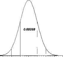
between ±1 is 0.68268. With the same probability the random variable x lies between 1 x a. Figure 10.43 shows the normalized Gaussian density function. It is useful to visualize this so-called bell-shaped curve when you interpret your output. Applying Table 10.2 to our example, we expect that in 99.73% of occurrences the range error will be within 50 m.

Instead of using the standard deviation to classify the range error, we can also ask the question: what is the 50% probability error bound.7 Starting with Eq. (10.129), we look for the integration bounds ±z that contain 50% of the area under the normal density function

From the normal table we interpolate for the value of 0.5 and receive г = 0.6745. For any distribution characterized by erv, we obtain, based on г = x/er,, the so – called range error probable (REP)

REP = zax = 0.6745ctv

Notice that the REP of 50% embraces smaller bounds than the one-sigma error, which occurs with the probability of 68.268% according to Table 10.2.

As an example, a fighter aircraft prepares to attack a target 3 km downrange. The pilot estimates that, given his one-sigma INS error of 100 m, he has a 50:50 chance to deliver the weapon within ±67.45 m of the required release point. The bomb itself has a ballistic error of REP = 50 m. Because both errors are statistically independent, they can be root mean squared together to provide the 50% probability that the bomb will land within V67.452 + 502 = ±84 m down – and up-range of the target coordinates.

The cross-range error or, as it is called, the deflection error probable (DEP) is defined in the same fashion. Given the lateral one-sigma error ery, then

DEP = 0.6745ery (10.131)

If the range and deflection errors are given by the univariate measures REP and DEP, the implicit assumption is made that the error distributions in the two directions are uncorrelated. You need to judge if this simplistic approach is adequate. When you analyze MC runs, you are more likely to find that the range and deflection errors are correlated, i. e., that they have a bivariate distribution. We now turn to discuss measures of accuracy for these two-dimensional situations.

10.3.1.2 Bivariate Gaussian distribution. Suppose you developed an air – to-ground guided missile simulation with many error sources and uncertainties. Now you execute MC runs and record the impact points in the x and у directions. From this two-dimensional data set*i, yu*2 , уг!• ■ ■ у і.. .’,xnyn, you calculate the means p. x, /лу and standard deviations ax, oy. You can adapt Eq. (10.127) to this process

£"=і<л – РхУ

but you also have to check whether the data are cross correlated by calculating the covariance <r,,,

л у

Y! i=i(xi – іххУуі – м>-)

Take note that the covariance is formulated without the square root. It has the squared units of x and y. Similarly, the variances of x and у are their standard deviations squared er2 and er2. The correlation coefficient can be calculated from the standard deviations and the covariance

It assumes values between zero and one. Your data are uncorrelated if p = 0. In most cases they will be correlated, and you have to employ the two-dimensional Gaussian probability density function

as a model for the distribution of your data. Equation (10.134) portrays a bell­shaped surface over the x, у plane with its peak over the mean coordinates p. x and pty. A plane p(x, y) = const intersects the surface in the form of an ellipse. The

volume above the ellipse is the probability that a data pair x, у will appear within the confines of the ellipse. The variances and covariances establish a particular ellipse, which can be represented by the two-dimensional covariance matrix

It is a symmetric matrix, which can be diagonalized to obtain the major and minor axes of the ellipse. Once diagonalized in the new coordinate system (principal axes), the covariance is zero, and the data set has become uncorrelated.

When you analyze your impact points, it is helpful to draw so-called containment ellipses, centered on the mean values. They indicate to you the stretch of the data and the principal axes. The CADAC utility BIVAR, a subprogram of KPLOT, provides you with this display capability.

Sometimes, your customer may ask, “Could you boil down your misses into a single number?” Then you know that he is asking for the circular error probable CEP or the mean radial error (MRE). “No problem,” you say, “as long as you accept the simplifying assumptions.”

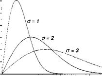
The definition of the CEP goes back to the times when the accuracy of rifles was determined by picking that circle on a paper target that contained 50% of the impact points. We take the mathematical approach and plot the radial distances r from the center as a histogram. If our simulation has enough noise sources with plenty of MC runs and the x and у dispersions are equal, we should see a density function similar to the Rayleigh distribution, also called the circular normal distribution. Its mathematical form is

p(r) = — e 2°r
W2

P(r)

0.6

ar is calculated from the data set r, Г2, .. ., r,-, .. . r„ by an equation similar to Eq. (10.127).

Once the probability density function is given, we can calculate the 50% probability from the distribution integral taken from zero to the median m

Take the natural logarithm on both sides and solve for m:

2

Cn 1 — Hn2 ——– m = ar^2 ft 2 = 1.1774<тг

2<Tf

The CEP is the median m, i. e., the 50% probability that an impact point will occur within a circle of the radius,

CEP = .llAor (10.137)

I have raised several warning flags that you must recognize in order to properly interpret your results. If you have some insurance that your simulation produces Gaussian distributions, you can apply the Rayleigh function. However, the CEP is only a good single number if the x and у means are near zero and the impact pattern is skewed no more than 2:1. It is always advisable first to plot the mean center and the elliptical distribution before calculating a single CEP number. You can do this with the CADAC/BIVAR program that plots impact points, the mean, ellipses with their major axes, and actually two CEPs, the aimpoint (target)-centered and the mean-centered CEP.

The MRE is not to be confused with the CEP, although their numerical values differ only by 7%. Given a one-dimensional density function p(r), the mean is the expectation integral

/

30

rp(r)dr

•OO

The MRE is the expectation integral of the Rayleigh distribution with r the distance of the impact point from the target. Its solution is given in integral tables

fx r2 І7Ґ

E{r) = / — e 2r, r dr — ar /— = 1.253orr

J-oо V 2

Therefore the MRE of a radial distribution, which conforms to the Rayleigh func­tion, is

MRE = 1.253e>y (10.138)

Compare Eq. (10.137) with Eq. (10.138) and note the slight difference of the two accuracy measures.

We have reached the end of our short tour of Monte Carlo. Although you did not get any help for improving your chances at the roulette table, I hope you are equipped to conduct and analyze your MC simulations. The univariate measures of merit, REP, DEP, and standard deviation portray range and deflection accuracy or one-sigma errors of each INS channel. They are the easiest to analyze. More difficult are the bivariate measures of merit, particularly if the data are highly skewed. In that case we have to work with elliptical distributions. However, the desire to interpret the accuracy by a single number leads to the reduction of the bivariate data to a single radial distribution and the definitions of CEP and MRE. You will have to judge under what circumstances this shortcut is advisable. Some practical applications should help you to sharpen your tools.