The centre-spring equivalent rotor

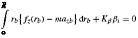
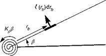
Reference to Fig. 3.6 shows that the equation of motion for the blade flap angle в (t) of the ith blade can be obtained by taking moments about the centre hinge with spring strength Kp; thus

(3.18)

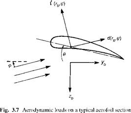
The blade radial distance has now been written with a subscript b to distinguish it from similar variables. We have neglected the blade weight force in eqn 3.18; the mean lift and acceleration forces are typically one or two orders of magnitude higher. We follow the normal convention of setting the blade azimuth angle, ф, to zero at the rear of the disc, with a positive direction following the rotor. The analysis in this book applies to a rotor rotating anticlockwise when viewed from above. From Fig. 3.7, the aerodynamic load fz(rb, t) can be written in terms of the lift and drag forces as

fz = —t cos ф — d sin ф t — dф

where ф is the incidence angle between the rotor inflow and the plane normal to the rotor shaft. We are now working in the blade axes system, of course, as defined in Section 3A.4, where the z direction lies normal to the plane of no-pitch. The acceleration normal to the blade element, azb, includes the component of the gyroscopic effect due to the

rotation of the fuselage and hub, and is given approximately by (see the Appendix, Section 3A.4)

azb ~ rb ^2fi( phw cos fi – qhw sin fi) + (qhw cos fi + phw sin fi) – & в –

(3.20)

The angular velocities and accelerations have been referred to hub-wind axes in this formulation, and hence the subscript hw. Before expanding and reducing the hub moment in eqn 3.18 further, we need to review the range of approximations to be made for the aerodynamic lift force. The aerodynamic loads are in general unsteady, nonlinear and three-dimensional in character; our first approximation neglects these effects, and, in a wide range of flight cases, the approximations lead to a reasonable prediction of the overall behaviour of the rotor. So, our starting aerodynamic assumptions are as follows:

(1) The rotor lift force is a linear function of local blade incidence and the drag force is a simple quadratic function of lift – both with constant coefficients. Neglecting blade stall and compressibility can have a significant effect on the prediction of performance and dynamic behaviour at high forward speeds. Figure 2.10 illustrated the proximity of the local blade incidence to stall particularly at rotor azimuth angles 90° and 180°. Without these effects modelled, the rotor will be able to continue developing lift at low drag beyond the stall and drag divergence boundary, which is clearly unrealistic. The assumption of constant lift curve slope neglects the linear spanwise and one-per-rev timewise variations due to compressibility effects. The former can be accounted for to some extent by an effective rotor lift curve slope, particularly at low speed, but the azimuthal variations give rise to changes in cyclic and collective trim control angles in forward flight, which the constant linear model cannot simulate.

(2) Unsteady (i. e., frequency dependent) aerodynamic effects are ignored. Rotor unsteady aerodynamic effects can be conveniently divided into two problems – one involves the calculation of the response of the rotor blade lift and pitching moment to changes in local incidence, while the other involves the calculation of the unsteady local incidence due to the time variations of the rotor wake velocities. Both require additional DoFs to be taken into account. While the unsteady wake effects are

accounted for in a relatively crude but effective manner through the local/dynamic inflow theory described in this section, the time-dependent developments of blade lift and pitching moment are ignored, resulting in a small phase shift of rotor response to disturbances.

(3) Tip losses and root cut-out effects are ignored. The lift on a rotor blade reduces to zero at the blade tip and at the root end of the lifting portion of the blade. These effects can be accounted for when the fall-off is properly modelled at the root and tip, but an alternative is to carry out the load integrations between an effective root and tip. A tip loss factor of about 3% R is commonly used, while integrating from the start of the lifting blade accounts for most of the root loss. Both effects are small and accounts for only a few per cent of performance and response. Including them in the analysis increases the length of the equations significantly however, and can obscure some of the more significant effects. In the analysis that follows, we therefore omit these loss terms, recognizing that to achieve accurate predictions of power, for example, they need to be included.

(4) Non-uniform spanwise inflow distribution is neglected. The assumption

of uniform inflow is a gross simplification, even in the hover, of the complex effects of the rotor wake, but provides a very effective approximation for predicting power and thrust. The use of uniform inflow stems from the assumption that the rotor is designed to develop minimum induced drag, and hence has ideal blade twist. In such an ideal case, the circulation would be constant along the blade span, with the only induced losses emanating from the tip and root vortices. Ideal twist, for a constant chord blade, is actually inversely proportional to radius, and the linear twist angles of O (10°), found on most helicopters, give a reasonable, if not good, approximation to the effects of ideal twist over the outer lifting portion of the blades. The actual non-uniformity of the inflow has a similar shape to the bound circulation, increasing outboard and giving rise to an increase in drag compared with the uniform inflow theory. The blade pitch at the outer stations of a real blade will need to be increased relative to the uniform inflow blade to produce the same lift. This increase produces more lift inboard as well, and the resulting comparison of trim control angles may not be significantly different.

(5) Reversed flow effects are ignored. The reversed flow region occupies

the small disc inboard on the retreating side of the disc, where the air flows over the blades from trailing to leading edge. Up to moderate forward speeds, the extent of this region is small and the associated dynamic pressures low, justifying its omission from the analysis of rotor forces. At higher speeds, the importance of the reversed flow region increases, resulting in an increment to the collective pitch required to provide the rotor thrust, but decreasing the profile drag and hence rotor torque.

These approximations make it possible to derive manageable analytic expressions for the flapping androtor loads. Referring to Fig. 3.7, the aerodynamic loads can be written in the form

where

We have made the assumption that the blade profile drag coefficient S can be written in terms of a mean value plus a thrust-dependent term to account for blade incidence changes (Refs 3.6,3.7). The non-dimensional in-plane and normal velocity components can be written as

Ut = гь(1 + rnxв) + д sin f (3.24)

Up = (д1 – Ло – вд cos f) + rb(Vy – в’ – Л1) (3.25)

We have introduced into these expressions a number of new symbols that need definition:

rb =	_ rb " R	(3.26)
uhw і д = Qr	1 2 1 2 1/2 uh + vh	(3.27)
(QR)2 )
ді =	whw ~QR	(3.28)

The velocities uhw, vkw and wbw are the hub velocities in the hub-wind system, oriented relative to the aircraft x-axis by the relative airspeed or wind direction in the x-y plane. в is the blade flap angle and 9 is the blade pitch angle. The fuselage angular velocity components in the blade system, normalized by Q R, are given by

Vx = Phw cos fі – qhw sin fі

Vy = phw sin fi + qhw cos fi (3.29)

The downwash, Л, normal to the plane of the rotor disc, is written in the form of a uniform and linearly varying distribution

vi

Л == Л0 + M(f )rb (3.30)

Q R

This simple formulation will be discussed in more detail later in this chapter.

We can now develop and expand eqn 3.18 to give the second-order differential equation of flapping motion for a single blade, with the prime indicating differentiation with respect to azimuth angle f:

Kp IpQ.[1] [2] ’

R jmr[3] dr o

derived directly from the hub stiffness and the flap moment of inertia Ip

where ao is the constant blade lift curve slope, p is the air density and c the blade chord.

Writing the blade pitch angle 9 as a combination of applied pitch and linear twist, in the form

9 = 9 p + rb9tw (3.33)

we may expand eqn 3.31 into the form

p” + fp’ Yp’ + (^2p + YH cos fife) Pi =

2((Tw + – w) cos fi – (vw – j sin ftj

+ Y f9p9p + f9tw9tw + fX(Hz — X0) + frn(®y — X1^ (3.34)

where the aerodynamic coefficients, f, are given by the expressions

1 + 3 H sin fi fp’ = 8	(3.35)
4 + 2h sin fi fp = fx = 1——- ^———	(3.36)
1 + 3 h sin fi + 2h2 sin2 fi f. p = 8	(3.37)
4 + 2h sin fi + 3 h2 sin2 fi f9 tw = 8	(3.38)
^ 1 + 3 H sin fi U = 8	(3.39)

These aerodynamic coefficients have been expanded up to O (h2); neglecting higher order terms incurs errors of less than 10% in the flap response below h of about 0.35. In Chapter 2, the Introductory Tour of this subject, we examined the solution of eqn 3.34 at the hover condition. The behaviour was discussed in some depth there, and to avoid duplication of the associated analysis we shall restrict ourselves to a short resume of the key points from the material in Chapter 2.

lag, but even the Lynx, with its moderately stiff rotor, has about 80° of lag between cyclic pitch and flap. The phase lag is proportional to the stiffness number (effectively the ratio of stiffness to blade aerodynamic moment), given by

(3)

There is a fundamental rotor resistance to fuselage rotations, due to the aerodynamic damping and gyroscopic forces. Rotating the fuselage with a pitch (q) or roll (p) rate leads to a disc rotation lagged behind the fuselage motion by a time given approximately by (see eqn 2.43)

Hence the faster the rotorspeed, or the lighter the blades, for example, the higher is the rotor damping and the faster is the disc response to control inputs or fuselage motion.

(4) The rotor hub stiffness moment is proportional to the product of the spring strength and the flap angle; teetering rotors cannot therefore produce a hub moment, and hingeless rotors, as on the Bo105 and the Lynx, can develop hub moments about four times those for typical articulated rotors.

(5) The increased hub moment capability of hingeless rotors transforms into increased control sensitivity and damping and hence greater responsiveness at the expense of greater sensitivity to extraneous inputs such as gusts. The control power, or final steady-state rate per degree of cyclic, is independent of rotor stiffness to first order, since it is derived from the ratio of control sensitivity to damping, both of which increase in the same proportion with rotor stiffness.

(6) The flapping of rotors with Stiffness numbers up to about 0.3 is very similar – e. g., approximately 1 ° flap for 1 ° cyclic pitch.

The behaviour of a rotor with Nb blades will be described by the solution of a set of uncoupled differential equations of the form eqn 3.34, phased relative to each other. However, the wake and swash plate dynamics will couple implicitly the blade dynam­ics. We return to this aspect later, but for the moment, assume a decoupled system. Each equation has periodic coefficients in the forward flight case, but is linear in the flap DoFs (once again ignoring the effects of wake inflow). In Chapter 2, we examined the hover case and assumed that the blade dynamics were fast relative to the fuselage motion, hence enabling the approximation that the blade motion was essentially pe­riodic with slowly varying coefficients. The rotor blades were effectively operating in two timescales, one associated with the rotor rotational speed and the other asso­ciated with the slower fuselage motion. Through this approximation, we were able to deduce many fundamental facets of rotor behaviour as noted above. It was also highlighted that the approximation breaks down when the frequencies of the rotor and fuselage modes approached one another, as can happen, for example, with hingeless rotors. This quasi-steady approximation can be approached from a more general per­spective in the forward flight case by employing the so-called multi-blade coordinates (Refs 3.4, 3.8).