Flight Dynamics

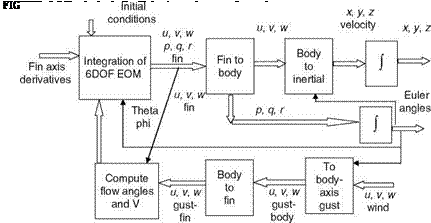
The flight dynamics of a vehicle to be simulated should be fairly accurately known. It is important to know the aerodynamic coefficients at all the flight conditions in the aircraft flight envelope. These are obtained from the wind-tunnel aero database and by application formulae. The EOMs are given in Chapter 3, and axes-transformation relations are given in Appendix A. Figure 6.5 depicts a flight dynamics simulation block diagram for a typical missile. The fin axis aerodynamic derivatives are first specified. The fin to body (noted as ‘‘b — f’’) transformation is done using the following matrix (angle f is generally 45 °):

1 0 0 0 cos w — sin w 0 sin w cos w

Body velocities are converted to inertial by using the direction cosine matrix. The inverse transformation is obtained by transposition of the respective matrices. The deterministic gust effects are transformed to fin axis for flight simulation. For numerical integration of nonlinear flight dynamics, generally the Runge-Kutta (R-K) method is used. It works well for a good number of such simulation problems, even with moderate discontinuities. In fact, it approximates the Taylor series method. Certain aircraft flight simulation aspects are illustrated by Examples 6.1 and 6.2, which demonstrate the complexity of the problem. Development of complete flight simulation is a highly complicated process.