Computation of Linear Models for Control Law Design

Not always, but more often than not, it is wiser and simpler to use the linear approach for the design of control laws. For this, one needs the linear dimensional models of the aircraft dynamics at several flight conditions in the flight envelope. These linear models are computed by a sophisticated program within the structure of nonlinear flight simulation, which uses aero database. The linear models are obtained by specifying Mach number, trim angle of attack, altitude, slat deployment, if any, and undercarriage up or down position. The linear simulation software would give linearized models along with the modal characteristics like eigenvalues and damping ratios of the longitudinal and lateral-directional modes (Chapter 5). Several thousand linear models would be required because of the variety of flight conditions and configurations in the entire flight envelope, as can be seen from the application formula. These linear models are then studied to arrive at important flight mechan­ics parameters (Chapters 4 and 8). It is important to evaluate the flight mechanics parameters of the aircraft from the aero database to assess the need for control-law design. These parameters would help assess the aircraft’s capability as well as deficiencies in the dynamics. These deficiencies could then be compensated by designing proper flight-control algorithms/laws/systems. Also, it is important to evaluate the dynamic characteristics and responses of the aircraft and study its handling qualities with flight simulation exercises while in the process of develop­ment of the aircraft (program). The flight mechanics parameters and linear models of the aircraft can be obtained using the equilibrium analysis of the aircraft dynamics.

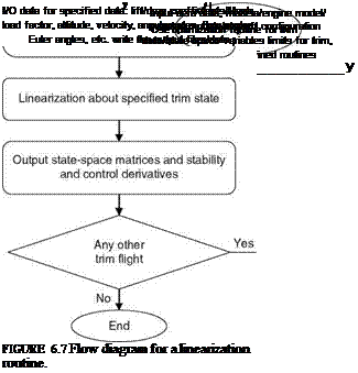
In fact, an aircraft is required to be trimmed for a given flight condition and then the linearization routine is used to obtain linear models at these flight conditions. Figures 6.6 and 6.7 give the flow diagrams of these routines. The derivation and development of linear models for an aircraft and related programming aspects are detailed in Refs. [16,17]. Such a program would consist of several modules [14] for (1) input data, (2) aerodata, (3) aerodynamic models, (4) engine model, (5) trim routine that would satisfy the required trim constraints according to the trim condi­tions set. This routine would also convert the trim parameters to control surface deflections, and (6) output results module, which will give the linear model stability and control derivatives, all the state-space matrices, and modal parameters of the aircraft dynamics at the chosen flight conditions.

The linearization can be done using the finite difference method. Let the non­linear equation for the aircraft dynamics be given as

Define a certain operating point as x0 = f(x0, u0) and use Taylor’s series linearization to obtain

df df

x(t) ffi x0 + (x — x0) + (u — u0) + (higher-order terms neglected)

dx du

df _ df _

x(t) — JC0 = ~ + u

dx du

The linearized equations would be represented as

x(t) = A’x + B U (6.30)

The numerical linearization routine would obtain the elements of the matrices A’, B’, (and C’, D’ of measurement equation) using a finite difference method, as shown for matrix A below:

(6.31)

Similarly for matrix B, the point (x0) is kept fixed and the point (u0) is perturbed by a term (Au,) for each element appropriately. A similar procedure can be followed to obtain the elements of the linearized measurement matrices C’ and D’. The step size for evaluating the numerical difference is typically given as

Ax, ! 10-7* x,

Forward differencing has been found to be quite accurate for the numerical compu­tation. Alternatively, a fixed value of 10e — 7 can also be used for the step size.