Axis Boundary Treatment

There are many aeroacoustics problems for which the use of a cylindrical coordinate system is the most natural choice for computing the solution. A simple example is the case of computing the noise from a circular jet. Another example is the numerical calculation of the propagation of acoustic waves inside a circular duct. The governing equations are the Navier-Stokes equations. When written in cylindrical coordinates, some terms of these equations with 1 /r coefficient apparently could blow up at the axis. In other words, there is an apparent singularity (although not a true one) at the axis (r = 0) of the coordinate system. In this section, a way to treat such apparent singularity is discussed.

9.4.1 Linear Problem Involving a Single Azimuthal Fourier Component

Acoustic problems are often linear. If the problem is linear and involves only a single azimuthal Fourier component, say the nth mode, then usually it is advantageous to separate out the azimuthal dependence by assuming that all variables have the dependence of єтф. On factoring out єтф, the reduced set of equations effectively becomes two-dimensional. Let the mean flow be axisymmetric. Near the x-axis, the mean flow may be assumed to be locally uniform; i. e., u = U, v = w = 0, p = p, p = p, and T = T. The linearized equations of motion are

+u +pv ■ v =0 (912)

¥ + = -1 vP + v v2v (9’13)

+4X) + pv- v=*tv2 T (914)

p = pRT + p RT, (9.15)

where vt and kt are the turbulent kinematic viscosity and thermal conductivity, if the flow is turbulent; otherwise, the molecular values should be used.

It can easily be shown that when Eqs. (9.12) to (9.15) are written in cylindrical coordinates (r, ф, x), it is an eighth-order differential system in r. Four of the solutions are bounded at r = 0. The other four are unbounded. Here, interest is confined to the bounded solutions alone.

In general, the velocity vector may be represented by a scalar potential Ф and vector potential A, that is,

v = vФ + v x A. (9.16)

For Eqs. (9.12) to (9.15), the solutions for the scalar and vector potentials can be obtained separately. It turns out that the viscous solutions are related only to the

vector potential. For convenience, the vector potential solutions will be referred to as viscous solutions.

Substituting Eq. (9.16) into Eqs. (9.12) to (9.15), it is easy to find that the governing equations for the scalar and vector potentials are

and

The viscous solutions are given by p = p = T = 0, v = Vx A.

9.4.1.1 Scalar Potential Solutions

General solutions of the scalar potential, Ф, may be found by applying Fourier – Laplace transforms to x and t and expanding ф dependence in a Fourier series, that is,

This reduces Eqs. (9.17) to (9.20) to a fourth-order differential system in r. The two solutions bounded at r = 0 may be expressed in terms of Bessel functions of order n. The complete solutions when written out in full are as follows:

un = ikJn (l■±r)- Vn = drrJn (X±r)

pn = p D’ (to — uk) — vt (4 + k2)] Jn (^±r)

where

ikt (to — uk)/R — p — cvpT + icVpvt [(to — uk)/R]
kt [vt/R + iT/(to — uk)]

—cvp(to — uk)2
Rkt [vt/R + iT/(to — uk)]

9.4.1.2 Viscous Solutions

There are two sets of viscous solutions. The first set is found by letting

A = ф ex, p = p = T = 0, (9.24)

where ex is the unit vectors in the x direction. Again, by the use of Fourier-Laplace transforms and Fourier expansion, the solution that is bounded at r = 0 is

Wn d/n[10]

p n pn Tn un 0

On following these steps, the bounded solution, after some algebra, is found to be

pn = pn = Tn = 0

9.4.1.3 Analytic Continuation into the r < 0 Region

The general solution is a linear combination of the scalar and vector potential solu­tions. The Bessel functions of these solutions can be continued analytically into the nonphysical region r < 0. For positive r, the analytic continuation formula for integer-order Bessel function is

Jn (—£r) = (—1)nJn (£r). (9.98)

By means of Eq. (9.98) and the preceding general solutions, it is straightforward to establish that

Pn (—r, x, t) = ( —1)n Pn (r, x, t)

p. n (—r, x, t) = ( — 1)npn (r, x, t)

Tn (—r, x, t) = (—1)n Tn (r, x, t) un (—r, x, t) = (—1)n un (r, x, t)

Vn (—r, x, t) = ( — 1)n+1 Vn (r, x, t) Wn (—r, x, t) = ( — 1)n+1 Wn (r, x, t),

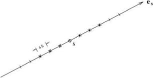
Figure 9.5. Approximating directional derivative in the es direction at і by a 7-point stencil finite difference quotient.

where pn, pn, etc. are the amplitude functions of the Fourier series expansions in ф.

Now, Eq. (9.29) may be used to extend the solution into the nonphysical negative r region to facilitate the computation of high-order large-stencil finite difference in r for points adjacent to the jet axis. That is, when a finite difference stencil extends into the negative r region, the values of the variables are found by Eq. (9.29). It is noted, however, that for n = 1,

lim v1 (r, x, t) = 0, lim w1 (r, x, t) = 0,

r^0 r^0

in general. For this reason, terms such as v1/r and w1/r cannot be computed at the jet axis r = 0. It is recommended that the values of v and w and all the other variables not be computed directly by the finite difference marching scheme at r = 0. Instead, the numerical solution at a new time level for all the other mesh points is first computed. The values of all the variables on mesh points in the region r < 0 is then calculated by analytical continuation. This leaves the values at r = 0 still to be determined. Here, it is suggested that they are to be found by high-order symmetric interpolation (see Chapter 11). Once the values of all physical variables at the axis r = 0 are found, the computation at the new time level is completed.