Beyond Level 1 Modelling

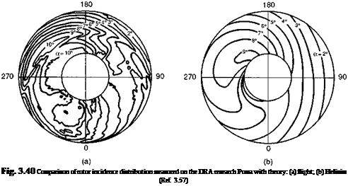
‘Theory is never complete, final or exact. Like design and construction it is continu­ally developing and adapting itself to circumstances’. We consider again Duncan’s introductory words and reflect that the topic of this final section in this model-building chapter could well form the subject of a book in its own right. In fact, higher levels of modelling are strictly outside the intended scope of the present book, but we shall attempt to discuss briefly some of the important factors and issues that need to be con­sidered as the modelling domain expands to encompass ‘higher’ DoFs, nonlinearities and unsteady effects. The motivation for improving a simulation model comes from a requirement for greater accuracy or a wider range of application, or perhaps both. We have already stated that the so-called Level 1 modelling of this chapter, augmented with ‘correction’ factors for particular types, should be quite adequate for defining trends and preliminary design work and should certainly be adequate for gaining a first-order understanding of helicopter flight dynamics. In Chapters 4 and 5 comparison with test data will confirm this, but the features that make the Level 1 rotor modelling so amenable to analysis – rigid blades, linear aerodynamics and trapezoidal wake struc­ture – are also the source of its limitations. Figure 3.40, for example, taken from Ref. 3.57, compares the rotor incidence distribution for the Puma helicopter (viewed from below) derived from flight measurements of rotor blade leading edge pressure, with the Level 1 Helisim prediction. The flight condition is a straight and level trim at 100 knots. While there are similarities in the two contour plots, theory fails to capture many of the details in the flight measurements. The region of high incidence on the retreating side is more extensive and further outboard in the flight results, and there is a clearly defined ridge in the flight measurement caused by the blade vortex interaction, which is, of course, completely missed by Helisim. At this 100-knot trim condition, Helisim may well predict the controls to trim reasonably accurately, simply because the integrated forces and moments tend to smooth out the effects of the detailed dif­ferences apparent in Fig. 3.40. However, there are a wide range of problems where the details become significant in the predictive capability of modelling. Examples include the pitch-up effect of blade stall in ‘high g’ manoeuvres, the transient rotor torque ex­cursions in rapid rolls, the effects of blade icing or battle damage on power and control

margins. If we consider the effects of the rotor wake on the tail rotor and empennage, then the simple trapezoidal downwash model fails to predict important effects, for example tail rotor control margins in quartering flight or the strong couplings induced by the wake effects on the rear fuselage and empennage, particularly in manoeuvres. High-fidelity simulation requires that these effects can be predicted, and to achieve this we need to consider the modelling elements at Levels 2 and 3, as described in Table 3.1. The following qualitative discussions will draw heavily from the published works of selected contributors to the field of enhanced rotorcraft modelling. The author is all too aware of the enormous amount of published work and achievements by a great number of researchers in Europe and the United States in recent years, particularly to rotor aeroelastic modelling, and a complete review is surely the topic for another text. The aim here is to draw the readers’ attention to selected advances that lay emphasis on physical understanding.