R Derivative of the Velocity Field

Let the (x, r, ф) components of the velocity field be denoted by (u, v, w). The r derivative of u at points near the cylindrical axis may be treated exactly the same as if u is a scalar. However, care must be exercised in forming the finite difference approximation for dr and fw.

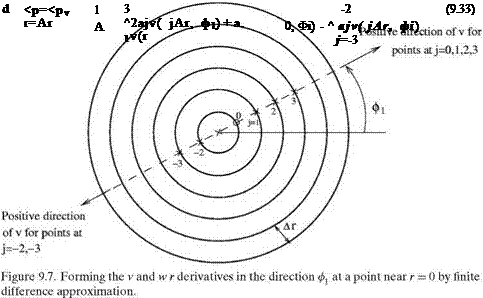
In a cylindrical coordinate system, v is positive in the positive direction of r. Now, to form a finite difference quotient to approximate the r derivative of v for a point at r = Ar in the direction of ф1, a 7-point symmetric stencil will extend to the other side of the origin at r = 0 as shown in Figure 9.7. For the points beyond r = 0, positive v is in the opposite direction. So, for the purpose of forming a directional derivative, we must use – v for these points. Hence,

Similar reasoning leads to the formula for dr as follows:

9.4.2.5 The Values of v and w at r = 0

The cylindrical axis is a singular line of the cylindrical coordinates. All the other points have a v and w velocity component. However, at r = 0, there is no radial or any azimuthal velocity component. In the r – ф plane, there is only a velocity vector vr=0 at r = 0.

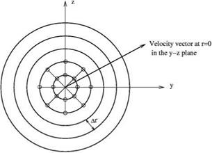
At r = 0, the cylindrical coordinate system is singular. It is not recommended to compute the velocity vr=0 by means of the governing equations of motion. A good approximation is to determine vr=0 by interpolation from values of v and w of the first few rings of points around the origin r = 0 (see Figure 9.8). For mesh

Figure 9.8. Determination of v at r = 0 by interpolation using values of (v, w) at mesh points in the first or first two rings.

points at angle ф = ф1 and r = nAr, the velocity components in the directions of the cylindrical coordiates and in the y and z direction are related by

vy = v cos ф1 – w sin ф1; vz = v sin ф1 + w cos ф1.

Now, the value of vy and vz at r = 0 may be taken, as a first approximation, to be equal to the average of the values of vy and vz at all the mesh points of the first ring. A more accurate value of these two quantities may be obtained by applying the multidimensional interpolation procedure of Chapter 13 to the values at the mesh points on the first two rings of the grid.