Stoke’s Theorem

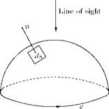
Stoke’s theorem relates the surface integral over an open surface to a line integral along the bounded curve. Let S be a simply connected surface, which is otherwise of arbitrary shape, whose boundary is c, and let u be any arbitrary vector. Also, we know that any arbitrary closed curve on an arbitrary shape can be shrunk to a single point. The Stoke’s integral theorem states that:

“The line integral J u ■ dx about the closed curve c is equal to the surface integral JJ (v x u) ■ nds over any surface of arbitrary shape which has c as its boundary."

That is, the surface integral of a vector field u is equal to the line integral of u along the bounding curve:

where dx is an elemental length on c, and n is unit vector normal to any elemental area on ds, as shown in Figure 5.17.

Stoke’s integral theorem allows a line integral to be changed to a surface integral. The direction of integration is positive counter-clockwise as seen from the side of the surface, as shown in Figure 5.17.

Helmholtz’s first vortex theorem states that:

“the circulation of a vortex tube is constant along the tube."

A vortex tube is a tube made up of vortex lines which are tangential lines to the vorticity vector field, namely curl u (or f). A vortex tube is shown in Figure 5.18. From the definition of vortex tube it is evident

curl u

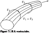that it is analogous to the streamtube, where the flow velocity is tangential to the streamlines constituting the streamtube. A vortex line is therefore related to the vorticity vector in the same way the streamline is related to the velocity vector. If Zx, Zy and Zz are the Cartesian components of the vorticity vector Z, along x-, y – and z-directions, respectively, then the orientation of a vortex line satisfies the equation:

along a streamline. In an irrotational vortex (free vortex), the only vortex line in the flow field is the axis of the vortex. In a forced vortex (solid-body rotation), all lines perpendicular to the plane of flow are vortex lines.

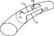
Now consider two closed curves c1 and c2 in a vortex tube, as shown in Figure 5.19.

According to Stoke’s theorem, the two line integrals over the closed curves in Figure 5.19 vanish, because the integrand on the right-hand side of Equation (5.13) is zero, since curl u is, by definition, perpendicular to n. The contribution to the integral from the infinitely close segments c3 and c4 of the curve cancel each other, leading to the equation:

u ■ dx + / u ■ dx = 0,

c1 J c2

since the distance between the segments c3 and c4 are infinitesimally small, we ignore that and treat c1 and c2 to be closed curves. By changing the direction of integration over c2, thus changing the sign of the second integral in Equation (5.14), we obtain Helmholtz’s first vortex theorem.
(5.15)
Derivation of this equation clearly demonstrates the kinematic nature of Helmholtz’s first vortex theorem. Another approach to the physical explanation of this theorem stems from the fact that the divergence of the vorticity vector vanishes. That is, the vorticity vector field curl u can be considered as analogous to an incompressible flow (for which the divergence of velocity is zero). In other words, the vortex tube becomes the streamtube of the new field. Now applying the continuity equation in its integral form (that is, JJs puiUi ds = 0) to a part of this streamtube, and at the same time replacing u by curl u, we get.
p (curl u) ■ nds = 0.
Since p is a constant, we can write this as.
(5.16)
(curlu) ■ nds = 0,
that is, for every closed surface s, the flux of the vorticity is zero. Applying Equation (5.16) to a part of the vortex tube whose closed surface consists of the surface of the tube and two arbitrarily oriented cross-sections A1 and A2, we obtain.
	(5.17)
since the integral over the tube surface vanishes. The integral.
(curlu) ■ nds
is called the vortex strength. It is identical to the circulation. From Equation (5.17) it is evident that. “the vortex strength of a vortex tube is constant." Noting the sense of integration of the line integral, Stoke’s theorem transforms Equation (5.17) into Helmholtz’s first theorem [Equation (5.15)]. From this representation it is obvious that, just like the streamtube, the vortex tube also cannot come to an end within the fluid, since the amount of fluid which flows through the tube (in unit time) cannot simply vanish at the end of the tube. The tube must either reach out to infinity (that is, should extend to infinity), or end at the boundaries of the fluid, or close around into itself and, in the case of a vortex tube, form a vortex ring. A very thin vortex tube is referred to as a vortex filament. The vortex filaments are of particular importance in aerodynamics. For a vortex filament the integrand of the surface integral in Stoke’s theorem

[Equation (5.13)]:

can be taken in front of the integral to obtain:

(curl u) • nAs = Г (5.19)

or

2a • n As = 2a As = constant, (5.20)

where a is the angular velocity. From this it is evident that the angular velocity increases with decreasing cross-section of the vortex filament.

It is a usual practice to idealize a vortex tube of infinitesimally small cross-section into a vortex filament. Under this idealization, the angular velocity of the vortex, given by Equation (5.20), becomes infinitely large. From the relation:

a As = constant,

we have a ^ ж, for As ^ 0.

The flow field outside the vortex filament is irrotational. Therefore, for a vortex of strength Г at a particular position, the spatial distribution of curl и is fixed. In addition, if div и is also given (for example, div и = 0 in an incompressible flow), then according to the fundamental theorem of vortex analysis, the velocity field и (which may extend to infinity) is uniquely determined provided the normal component of velocity vanishes asymptotically sufficiently fast at infinity and no internal boundaries exist.

The fundamental theorem of vector analysis is also essentially purely kinematic in nature. Therefore, it is valid for both viscous and inviscid flows, and not restricted to inviscid flows only. Let us split the velocity vector и into two parts, namely due to potential flow and rotational flow. Therefore:

U — Uir + Ur, (5.22)

where u! R is velocity of irrotational flow field and uR is velocity of rotational flow field. Thus, u! R is velocity of an irrotational flow field, that is:

curl u! R = v x uR = 0, (5.23)

The second is a solenoidal (coil like shape) flow field, thus:

divuR = v • uR = 0. (5.24)

Note that Equation (5.23) is the statement that “the vorticity of a potential flow is zero” and Equation (5.24) is the statement of continuity equation of incompressible flow.

The combined field is therefore neither irrotational nor solenoidal. The field u! R is a potential flow, and thus in terms of potential function ф, we have u! R = v ф. Let us assume that the divergence u to be a given function g(x). Thus:

div u — v • uir + v • ur — g(x),

div u = v • uir = g(x),

since v • uR = 0. Also, u! R = v ф. Therefore: