Scattering by Very Thin Axial Splices

This example involves acoustic mode scattering by two thin axial splices. The com­putational model is shown in Figure 10.13. The same computational grid (see Figure 10.15) as in the previous subsection is used. The azimuthal mesh size of the outer­most ring of the cylindrical mesh is equal to 0.0123. Here, the acoustic scattering by two thin hard wall splices with a width of 0.006 is studied. It is noted that the splice width is approximately half of that of the mesh spacing (see Figure 9.15). In other words, the splices are invisible to the discretized computation.

Consider the periodic function, О(ф), of period 2п, defined by

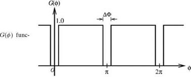°, -1АФ <ф<М п — Аф<ф<п + Аф

Ь(ф) =

1, otherwise

where АФ is the angle subtended by a splice. A graph of О(ф) is shown in Fig­ure 10.18. When applied to the surface of the duct, О(ф) = 1 where there is acoustic liner. It is equal to zero where there is hard wall splice. By means of the G-function, the wall boundary condition in the duct may be written as

Now, G^) is a period function; it may be expanded as a Fourier series. It is easy to find that

TO

G(ф) = ^ aj cos (]ф),
j=0

where

It is clear from Fourier expansion (10.52) that the G^) function contains compo­nents that are beyond the resolution of the 7-point stencil DRP scheme. To compute

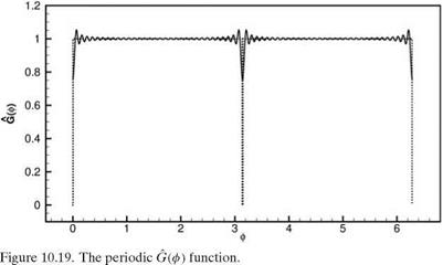acoustic wave propagation in the duct, these high wave number components essen­tially make the splice invisible to the computational mesh. A simple way to make the spliced liner compatible with the numerical scheme is to remove all Fourier components with azimuthal wavelengths shorter than the cutoff wavelength of the computational algorithm. Accordingly, all Fourier components with mode number m larger than mc, where the wavelength of mode mc is the same as or is closest to the smallest resolved wavelength of the computation scheme. For the cylindrical mesh used in the present computation, the azimuthal mesh size at the outermost ring is equal to 0.0123. For the 7-point stencil DRP scheme, acAx = 1.2, so that ac = 1.2/0.0123 = 97.6. Hence, by equating mc to the integer value closest to ac/2, it is found that mc = 49. Figure 10.19 shows the graph of the truncated Fourier series, G(ф) (Fourier components with m greater than 49 are removed), i. e.,

m

c

G(ф) = ^2 aj cos(]ф). (10.54)

m=0

The modified spliced liner boundary condition is to replace Є(ф) by G (ф) in Eq. (10.51), i. e.,

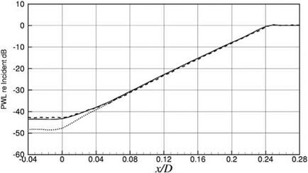
Figure 10.20 shows three computed PWL distributions along the length of the duct for the same incident duct mode as Section 10.6.1. In this computation, boundary condition (10.48) is used in the neighborhood of the liner hard wall junction at the two ends of the computational model. The dotted line in Figure 10.20 shows the numerical result when boundary condition (10.51) is used. There is no scattering in this case because the splices are invisible to the computational mesh. The full line is the computation using modified boundary condition (10.55). There is a large difference between these two curves. The difference is the energy of the scattered waves that are clearly quite substantial at the duct inlet. To check the accuracy of the wave number truncation method, a third computation using the quasi-two-dimension

Figure 10.20. Axial distribution of PWL. Incident wave has azimuthal mode number m = 26, radial mode number n = 1, angular frequency Q = 0.573. Liner impedance Z = 2 + i (time factor e-iQt). Ax = 0.008.——– , computed by boundary condition (10.55);—————————————- computed by boundary condition (10.51);——- , computed by Fourier expansion method (89 modes) of Tam et al. (2008).

azimuthal mode expansion method of Tam et al. (2008). This method expands the propagating acoustic waves in a large number of azimuthal modes. For the present computation, modes up to (mc + 40) are included. As a result of the large number of modes, the computation requires very large computer memory and long CPU time. The dashed curve of Figure 10.20 is the computed result using this method. It is evident that the result is very close to that of the wave number truncation method. This example offers a rigorous test of the effectiveness and accuracy of the wave number truncation method for computing the scattering of acoustic waves by narrow scatterers.