Extrapolation Error in Wave Number Space

Now, instead of Lagrange polynomials extrapolation formula (11.2), a more general formula,

(n-1)

f (X0 + nAx) = J2 Sjf (Xj), Xj = X0 – jAx, (11.12)

j=0

will be used, where Sj (j = 0, 1, 2,…, N-1)) are the stencil coefficients. Sj is unknown at this stage and Sj is equal to ljn) (x0 + n Ax) for the Lagrange polynomial

extrapolation method. Now, the local extrapolation error for wave number aAx, Elocal(n, к, a Ax, N), is defined as the square of the absolute value of the difference between the left and right side of Eq. (11.12) when a single Fourier component of Eq. (11.11) is substituted into the formula as follows:

Note that Elocal(n, к, – a Ax, N) = Elocal(n, к, aAx, N).

The integrated error over the band of wave numbers from aAx = 0 to aAx = к

One expects the extrapolation error to be zero if the function is a constant or a = 0. From Eq. (11.13), this condition gives

fN-1

J2Si – ^ = °-

j=0

Now, Sj, the coefficients of extrapolation formula (11.12), is to be chosen so that E is a minimum subjected to constraint (11.15). This constrained optimization problem can easily be solved by the method of the Lagrange multiplier. The Lagrangian function may be defined as follows:

(11.16)

The coefficients Sj and the Lagrange parameter X are found by solving the linear system as follows:

Now, the integrals of Eq. (11.17) can be readily evaluated. The algebraic system of Eqs. (11.17) and (11.18) leads to the following linear matrix equation:

(11.19)

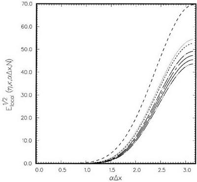
In Eq. (11.19), к is a free parameter. This parameter is to be selected so as to offer the best overall results. Once Sjs are found, the local error Elocal may be

computed according to Eq. (11.13). Figure 11.5 shows the dependence of E^ on wave number aAx in the case n = 0.75 and N = 7 for several values of к. This figure is typical of other values of n and N. Plotted in this figure is also the local error of the Lagrange polynomials extrapolation. It is readily seen that the Lagrange polynomials extrapolation is very accurate for low wave numbers, but the error becomes large for a Ax > 0.6 or wavelengths shorter than 10.5 Ax. Many finite difference schemes used in large-scale computations and simulations can resolve waves longer than eight mesh spacings or a Ax < 0.85. Therefore, it would be incompatible to use the Lagrange polynomials extrapolation with these schemes. On the other hand, the local error of the optimized extrapolation is larger at very low wave numbers. The error up to a Ax = 0.85 is quite comparable to those of the high-order computational schemes. Figure 11.6 shows the distribution of local error over the full range of wave numbers, i. e., 0 < a Ax < n. Note that at aAx = n, the local error of the Lagrange polynomials method is exceedingly large.

To examine the variation of extrapolation error on n, let

This is the maximum error incurred in the extrapolation process if the function involved has a Fourier spectrum confined to the range aAx < 0.85. Figure 11.7 shows the dependence of Emax on n for the case N = 7. For к = 0.85, is less than

Figure 11.6. Dependence of local error on wave number (full range) for the case n = 0.75, N = 7………….. , к = 0.8;——– , к = 0.85;——– , к = 0.95;——— , к = 1.0;……………………. , к = 1.05; ———— , к = 1.1;——– , Lagrange polynomials extrapolation.

10- 2 for n up to 1.0. A similar investigation for N = 5,6, and 8 shows that Emax remains low if к is taken to be 0.85. Based on this numerical study, it is recommended that the parameter к be assigned the value 0.85 when used in connection with large-scale high-order finite difference computation.