Airfoil Shape Effects: Sane’s Use of Polhamus’s Analogy

Figure 3.38 shows the normalized vorticity field around a SD7003 in deep stall, following the same kinematics as introduced in Section 3.5.1 at Re = 6.0 x 104. The phase-averaged field obtained using a 3D implicit filtered large-eddy simulation

xi/c = 0.125 0.25 0.5 0.75 0.25 behind TE

-10 12-1012-1012-1012-1012

Ui/U^l ‘иі/иж ui/U ж ‘иі/иж ui/U ж

t/T= 0.50 (bottom of the downstroke)

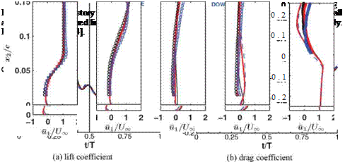
Figure 3.36. щ/U^ profiles from the numerical and experimental results at constant x1/cm = 0.125, 0.25, 0.50, 0.75, and 0.25 behind the trailing edge at t/T = 0.00 and 0.50 at Re = 1 x 104 (numerical: dashed line; experimental: square), 3 x 104 (numerical: dash-dotted line; experimental: cross), and 6 x 104 (numerical: solid line; experimental: circle) for the 2D flat plate in shallow stall. From Kang et al. [324].

-0.4 x/c

0

0.25

0

0.2

(a) implicit LES (b) PIV (c) RANS

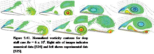
Figure 3.38. Normalized vorticity field around an SD7003 in deep stall. (a) Phase – and spanwise – averaged implicit LES computations by AFRL; (b) phase-averaged PIV measurements by AFRL; (c) RANS computation by University of Michigan. t/T = 0,0.25,0.5, 0.75. From Ol et al. [326].

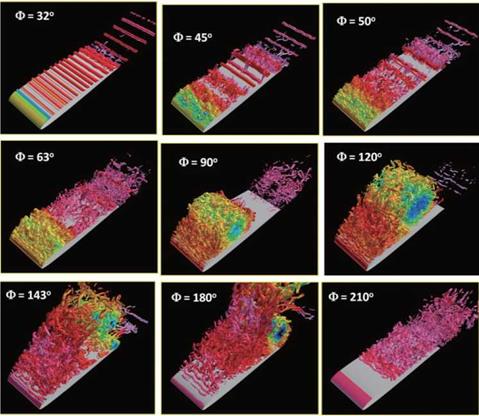
Figure 3.39. Instantaneous iso-Q-surfaces (Q = 500) colored with density showing 3D flow structures at selected phases (Ф) of the motion cycle computed using the implicit LES. From Visbal [327].

(LES), phase-averaged PIV, and 2D RANS solutions with Menter’s shear stress transport (SST) turbulence model is included as an example. As the airfoil plunges down, the flow on the suction side starts to separate, forming an LEV. At the bottom of the downstroke, the LEV is already detached, while a well-defined TEV is seen in both computations. A smaller TEV is observed at an earlier phase in the PIV measurements. The smaller details of each vortical structure are well illustrated by the implicit LES computations and the PIV measurements at this Reynolds number. The RANS solution, in contrast, gives a smoother flow field.

The qualitative agreement between the computational and the experimental approaches is better when the flow is largely attached. When the flow exhibits a mas­sive separation (t/T = 0.5), the experimental and computational results show notice­able differences in phase as well as the size of flow separation. Three-dimensional instantaneous flow structures are illustrated in Figure 3.39. The iso-Q-surfaces show the evolution of the vortical structures as computed using an implicit LES solver. At this Reynolds number, the flow during the downstroke and the first part of the upstroke is characterized by three-dimensional small vortical structures that form the LEV, which eventually convects away and breaks down. At the bottom of the downstroke, a well-defined TEV is also clearly visible. Figure 3.40 depicts the lift

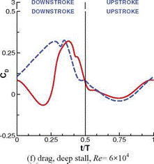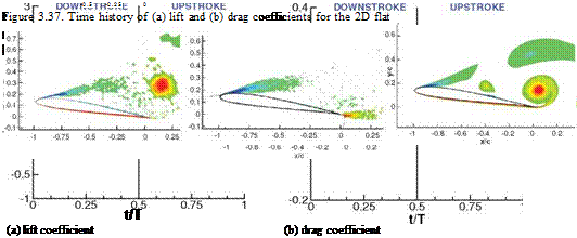
Figure 3.40. Time histories of forces on the 2D flat plate (dashed line) and SD7003 airfoil (solid line). From Kang et al. [324].

coefficient computed by the participating institutions for the same case. The upper bound is given by the quasi-steady equation, which is discussed in the next section. The RANS computations result in a smoother lift history than the implicit LES computation, reflecting the vorticity flow field shown in Figure 3.38. Note also that Theodorsen’s lift formula approximates the unsteady lift well (see Section 3.6).

As discussed in the introduction to Section 3.5, Kang et al. [324] investigated the effects of airfoil shapes for the same kinematics, the time histories of force coefficients, and the vorticity contours. Ol et al. [323] discussed in detail the flow physics for SD7003 airfoil at several Reynolds numbers. First, the comparisons of the computed force coefficients are shown in Figure 3.40 for Re = 1 x 104 and 6 x 104 for the flat plate and the SD7003 airfoil. It is clear that the flat plate shows greater lift peaks than the SD7003 airfoil within the range of Reynolds numbers and airfoil kinematics considered in their study [324]. Moreover, Baik et al. [325] observed a phase delay of the peak in the deep stall case at Re = 6 x 104 (see Fig. 3.40b). This is because the flow separates earlier over the flat plate during the downstroke. The corresponding normalized vorticity fields for the SD7003 and flat plate in the deep stall case are shown in Figure 3.41 during the downstroke. The vorticity distribution over the SD7003 airfoil is shown at t/T = 0.33, 0.42, and 0.50 (Fig. 3.41a) and for the flat plate at earlier time instants of t/T = 0.25, 0.33, and 0.42 (Fig. 3.41b). Due to the smaller radius of curvature at the leading edge of the flat plate, the flow around the leading edge experiences a stronger adverse pressure gradient, separating at a lower effective AoA. The leading-edge shear layer and the LEV on the suction side of the flat plate have similar topology to that of the flow field of SD7003 with a phase lag of approximately 0.083. As the LEV and the TEV detach from the airfoils, the difference in lift between these two airfoils diminish.

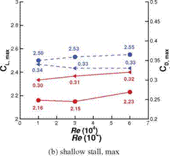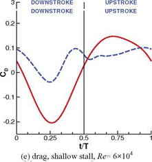
(c) deep stall, mean (d) deep stall, max

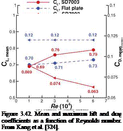
The mean and maximum force coefficients for both airfoil shapes for several Reynolds numbers are summarized in Figure 3.42. The geometric effect due to the sharper leading edge of the flat plate overwhelms the variations in motion kinemat­ics and Reynolds number: the maximum lift is obtained by the flat plate for both kinematics. Furthermore, the force coefficients of the flat plate are insensitive to the Reynolds number. It is also interesting to note that the mean drag coefficient is lower for the SD7003 airfoil because of its streamlined body and that the mean lift coefficient is higher for the SD7003 airfoil for Re = 3 x 104 and 6 x 104, when the flow is attached over most of the motion period.

Sane [312] discussed the effects of delayed stall and LEV on force generation using Polhamus’s analogy [321]. For airfoils without leading-edge separation, the flow over the leading edge accelerates and creates a suction force that is parallel to the chord. This suction force tilts the resulting force forward in the direction of thrust at low AoAs. For a flat plate the flow separates at the leading edge, and an LEV forms on the suction side. The LEV increases the force normal to the flat plate,

I ■

0 0.2 0.4 0.6 0.8 1 1.2 1.4

SD7003 t/T

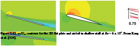
resulting in increased lift and drag for positive AoA. In this effort, for the shallow stall case, the SD7003 airfoil generates lower lift peak (Fig. 3.40a) but greater thrust compared to the flat plate due to attached flow and leading-edge suction (Fig. 3.40e). Figure 3.43 shows the normalized streamwise velocity contours around the 2D flat plate and the SD7003 airfoil at Re = 6 x 104 for the shallow stall case. During the downstroke the flow separates at the leading edge, forming an LEV that covers the whole suction surface of the flat plate, consistent with the higher lift peak and greater drag during the downstroke shown in Figure 3.40a and Figure 3.40e, while the flow over the SD7003 remains mostly attached. When the prescribed motion is more aggressive for the deep stall case, the flow over the SD7003 airfoil separates near the leading edge during the downstroke (Fig. 3.41), and the resulting lift and drag time histories are similar to those of the flat plate (Fig. 3.40b, f) for the period in which the flow is separated. There is still a significant difference in drag (Fig. 3.40f) during
the first portion of the downstroke, because the flow over the SD7003 airfoil separates later than over the flat plate. Hence, Sane’s application of Polhamus’ analogy is valid for the shallow stall motion and to a lesser extent for the deep stall motion. For motions with greater effective AoA, the flow over the blunt airfoil may separate, and then the resulting force on the blunt airfoil is qualitatively similar to that of a flat plate.