Spatial Stencils for Use in the Mesh-Size-Change Buffer Region

If a factor-of-2 increase in the mesh size between adjacent blocks is used, then every other mesh line in the fine mesh block continues into the coarse mesh block as shown in Figure 12.1. The remaining set of mesh lines terminates at the mesh-size-change interface. To compute the x derivative for points on the coarse grid, including points on the interface such as point A, the 7-point central difference DRP scheme may be used even though part of the stencil is extended into the fine mesh region. For mesh points on the fine grid, again the 7-point central difference DRP scheme may be used except for the first three columns (or rows) of mesh points right next to the coarse grid. For points on the continuing mesh lines such as points B and C in Fig­ure 12.1, special central difference stencils, as indicated, are to be used. These stencils may be written in the following form:

To find the stencil coefficients aBj and aCC (j = -3 to 3), the optimization procedure of Chapter 2 may be followed. Now, first consider the stencil for point B. As in Section 11.2, it will be assumed that f(x) has a Fourier transform f(a) with absolute value A (a) and argument ф(а); i. e.,

A(a) = | f(a)|, ф(а) = arg[ f(a)|.

The Fourier transform may be written as

f (x) = / A(a*"*-*d

In other words, f(x) is made up of a superposition of simple waves, fa(x), of the following form:

fa(x) = еТ“+ф(а)], (12.4)

weighted by A (a). Now the accuracy of finite difference approximation (12.1) of each simple wave component of f(x) is examined. Upon substituting fa (x) into Eq. (12.1), the finite difference approximation becomes

a fa(x) ~ a fa(x),

where

2

a = — aB sin (a Ax) + aB sin (3a Ax) + aB sin (5aAx)] (12.5)

is the wave number of the finite difference stencil. In deriving (12.5), the antisym­metric condition, a – j = – aB, has been invoked.

On following the steps of Chapter 2, the condition that Eq. (12.1) or Eq. (12.5) be accurate to order (Ax)4 is imposed. By means of Taylor series expansion, this condition yields the following restrictions on the stencil coefficients:

2(aB + 3aB + 5aB) = 1

aB + 33aB + 53 aB = 0 (12.6)

The coefficients will now be chosen so that the error of using a Ax to approximate a Ax over the band of wave number | a Ax| < к, E, is minimum subjected to conditions (12.6). For this purpose, the error is defined as к

J [aAx – aAx]d (a Ax) 0

The condition for a minimum is given by (after eliminating aB and a3B by Eq.

An extensive numerical study of the effects of the choice of к on a(a) and da /da has been carried out. Based on the numerical results, it is deemed that a good choice

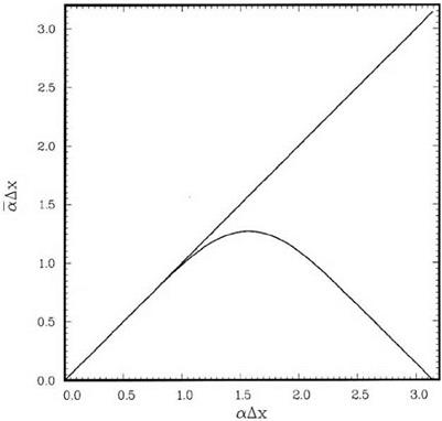
Figure 12.3. Dependence of a Ax on a Ax for stencil B. к = 0.85.

of the values of к is 0.85. For this choice, the values of the stencil coefficients are

aB = 0.0

aB = aB1 = 0.595328177715 aB = aB2 = -0.037247422191 a3B = aB 3 = 0.003282817772.

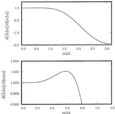
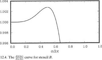
Figures 12.3 and 12.4 show the corresponding a(a) and dal da curves. The resolution and dispersion characteristics of the stencil lie in between those of the central difference DRP scheme on the two sides of the interface.

On proceeding as for stencil B, the stencil coefficients for stencil C may be found. For stencil C, it is recommended that the value к = 1.0 be used. The stencil coefficients are

aC = 0.0

aC = aCB1 = 0.726325187522 aC = aC2 = -0.120619908868 aC = aC3 = 0.003728657553.

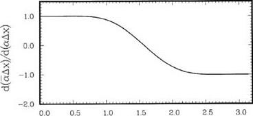
Figures 12.5 and 12.6 show the corresponding a(a) and da/da curves for this stencil. Again, the resolution and dispersion characteristics lie in between those of the central difference DRP scheme on the two sides of the interface.

аДх

Figure 12.6. The doff) curve for stencil C.

For mesh points lying on the terminating mesh lines such as points A’, B’, and C of Figure 12.1, the same stencils as for A, B, and C may be used, However, the stencils extend into points in the coarse mesh region where the solution is not computed. To obtain the values of the solution at these points, such as point D, it is recommended that interpolation be used. The interpolation stencil, a symmetric stencil is preferred, makes use of the values of the adjacent 6 mesh points, D1 to D6, as shown in Figure 12.1. In actual computation, the interpolation step is executed only after the solution on the coarse mesh region has been advanced by a time step. The interpolated values allow the solution on the fine mesh side to continue advancing in time.