FUZZY LOGIC CONTROL

Conventional control systems are not regarded as intelligent systems. If in conven­tional control strategy some logic is used, then it can be a start of the intelligent control system. Fuzzy logic provides this possibility. A fuzzy logic-based controller is suitable for keeping the output variables within the specified limits and also for keeping the control actuation, i. e., the control input and the related variables, within limits. In fact fuzzy logic deals with vagueness rather than uncertainty. Fuzzy logic in control would be useful if the system dynamics are slow or nonlinear, when models of the system are not available, and competent human operators are available to derive the expert rules [7]. Thus, the rule-based fuzzy system can model any continuous function or system and the quality of fuzzy approximation would depend on the quality of rules. These rules can be formed by experts and, if required, ANNs can be used to learn the rules from the empirical data. Such systems are called ANFIS (adaptive neuro-fuzzy inference system) (Chapter 9). The basic unit of the fuzzy system/approximation is the ‘‘If… Then… ’’ rule. A fuzzy variable is one whose values can be considered labels of fuzzy sets: temperature! fuzzy variable! linguistic values such as low, medium, normal, high, very high, etc. leading to membership values (on the universe of discourse, e. g., degree Celsius). The dependence of a linguistic variable on another variable can be described by means of a fuzzy conditional statement:

R: If S1 (is true), then S2 (is true) or S1 ! S2 (8.10)

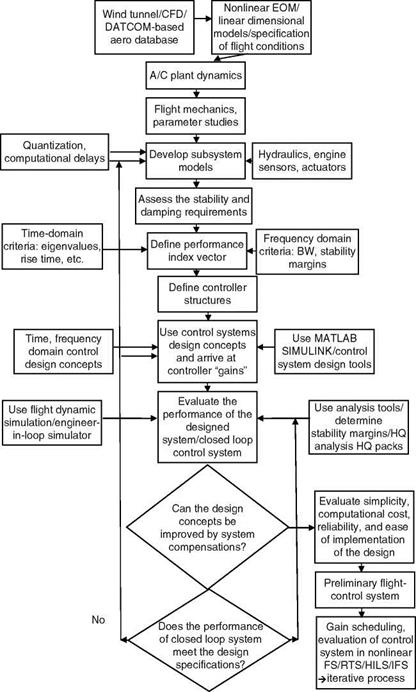
FIGURE 8.2 A typical iterative process for design of flight control.

FIGURE 8.3 Time histories of aircraft with destabilized controller (Example 8.3).

R1: If S1 then (If S2 then S3) is equivalent to: R1: If S1 then R2 AND R2: If S2 then S3

The number of rules could be large (30) or for a more complex process control plant 60 to 80 rules might be required [7]. For a small task 5 to 10 rules might be sufficient like for a washing machine. Then, a fuzzy algorithm is formed by combining 2 or 3 fuzzy conditional statements: If speed error is negative large then (if change in speed error is NOT [negative large or negative medium] then change in fuel is positive large), . . . , or, . . . , or, . . . .

The knowledge necessary to control a plant is usually expressed as a set of linguistic rules of the form: If (cause) then (effect). These are the rules that new operators are trained with to control a plant, and the set of rules constitutes the knowledge base of the system. However, all the rules necessary to control a plant might not be elicited or even known. It is therefore essential to use some technique capable of inferring the control action from available rules. Forward fuzzy reasoning (Generalized Modus Ponens):

Premise 1: x is A,

Premise 2: If x is A then y is B,

Then the consequence: y is B. This is the forward data-driven inference, used in all fuzzy controllers, i. e., given the cause infer the effect. The directly related to backward goal-driven inference mechanism, i. e., infer the cause that leads to a particular effect, is as follows:

Generalized Modus Tollens:

Premise 1: y is B,

Premise 2: If x is A then y is B,

Then the consequence: x is A. Reasons for use of fuzzy control are (1) for a complex system! the math model is hard to obtain, (2) it is a model-free approach, (3) human experts can provide linguistic descriptions about the system and control instructions, (4) fuzzy controllers provide a systematic method to incorporate the knowledge of human experts, and (5) it reduces the design iterations and simplifies the design complexity. It can reduce the hardware cost and improve the control performance, especially for the nonlinear control systems. The assumptions involved in a fuzzy logic control system are [7] (1) the plant is observable and controllable, (2) expert linguistic rules are available or formulated using engineering common sense, intuition, or an analytical model, (3) a solution exists, (4) it is sufficient to look for a good enough (approximate reasoning) solution and not necessarily the optimum one, (5) there is a desire to design a controller to the best of our knowledge and within an acceptable precision range, and (6) the problem of stability/optimality remains as an open issue. Heuristic knowledge-based control does not require deep knowledge of the controlled plant and this approach is popular in the industry and manufacturing environment where such knowledge is lacking. It is case dependent and does not resolve the issue of overall system’s stability and performance. Model-based fuzzy control (MBFC) combines the fuzzy logic and theory of modern control; especially the known model of the plant can be used. This approach is useful in the control of high-speed trains, in robotics, helicopters, and flight control. In the classical gain scheduling control, the control gains are computed as a function of some variable, e. g., the dynamic pressure at flight conditions. Fuzzy gain scheduling (FGS) is a special case of MBFC and uses linguistic rules and fuzzy reasoning to determine the control laws at various flight conditions. The issues of stability, pole placement, and closed loop dynamic behavior are resolved using the conventional and modern control approaches.

Tagaki and Sugeno (TS) [7] controller is defined by a set of fuzzy rules. These rules specify a relation between the present state of the dynamic system and its model and the corresponding control law with a general rule! R: If (state) Then (fuzzy plant/process model) AND (fuzzy control law).

Let the dynamic system be given as

X(t) = f (x, u); x(0) = X0 (8.12)

Define the fuzzy state variables for the discrete case as

fXj = Y^ mfXij(x)/x (8.13)

Each element of the crisp state variable is fuzzified and in each fuzzy region of fuzzy state-space the local process model is defined:

One example of fuzzy process rules is given in Example 8.4. The process rules can be given in terms of the elements of the crisp process state. The process is specified by the state space with the degrees of fulfillment of the local models of the process employing Mamdani rule.

x1 = mS (x)fi(x, u)

= min(mfx{ (X1),…, mfxn (Xn))fi(x, u)

The fuzzy open loop model is given as

-X = X w‘s(x)fi(x, u) (8.16)

is the normalized degrees of fulfillment. Now the fuzzy control

Rls: if x = fxl then u = g,(x) (8.17)

In a manner similar to the development of the fuzzy open loop/process model, the control law is defined as

u = X Wc(x)gj (x) (8.18)

Here, w are the control weights. An aircraft’s dynamic characteristics would change with Mach number and altitude (or dynamic pressure). Gain scheduling is used for selecting appropriate filter (feedback controllers) characteristics (gain and time constants) so that the performance of the aircraft/control system is acceptable despite the change in its dynamics. The concept is illustrated by the following example.

Example 8.4

Use the system process rules as [7]

R0: if xd = 0 then x = f1(x, u) = — 0.4x + 0.4u R1: if xd = 1 then x = f2( x, u) = —2.5x + 2.5u

Then

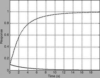
1. Obtain step responses of these two systems/process rules and compare the results.

2. Use the fuzzy gain scheduling controller concept with the following rules:

R0: if xd = 0 then u1 = g1(x, xd) = k1(x — x^)

R1: if xd = 1 then u2 = g2(x, xd) = k2(x — xd)

Use the state feedback gains кг = 0.5 and k2 = 0.92. Then the overall fuzzy process model is given by the weighted sum:

x = wi{-0.4(x — xd) + 0.4u} + w2{—2.5(x — xd) + 2.5u} (8.21)

Design the above fuzzy gain scheduling and obtain the responses of the final system.

3. Compare the responses of the designed system with the system: x = —0.2x + 0.2u.

4. Plot all the results: step responses and Bode diagrams of the open loop and closed loop systems.

Solution

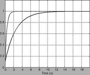
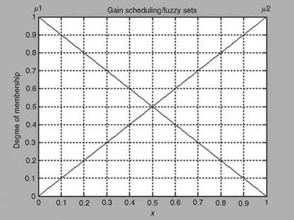
The process time constants are 2.5 and 0.4 s. The step responses of these processes are shown in Figure 8.4 (ExampleSolSW/Example8.4FuzzyControl). It is obvious from the plots that the second process rule signifies a faster process. The fading of the slow plant dynamics to the fast one is represented by the fuzzy membership functions plotted in Figure 8.5, as altitude increases. The fuzzy control law is given as

u = 0.5w1(x — xd) + 0.92w2 (x — xd) (8.22)

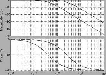
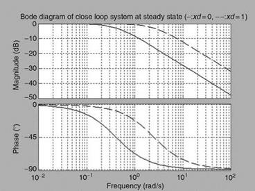
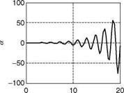
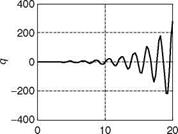
The Fuzzy controller is realized as discussed in Section 8.6, and the responses are shown in Figure 8.6. The comparison of the time responses with the invariant system is shown in Figure 8.7. The frequency responses for the open loop and closed loop systems are represented in Figures 8.8 and 8.9. The fuzzy controller meets the require­ments at both the ends as can be seen from Figure 8.7.

Response of system to unit step input (open-loop)

FIGURE 8.5 Gain scheduling fuzzy membership functions: Transition from slow dynamics to fast dynamics as the altitude increases.

Response of system with fuzzy feedback controller

Bode diagram of open loop system (-:xd =0, —:xd = 1) Frequency (rad/s)

FIGURE 8.9 Closed loop frequency responses of the system for two processes: At low altitude xd — 0 (- slow dynamics); at high altitude xd — 1 (— fast dynamics).

8.7 FAULT DETECTION, IDENTIFICATION, AND ISOLATION

In the present-day complex and sophisticated control systems for aerospace vehicles, the safety and reliability of the system are very important. A failure or fault could be in the hardware system or in the software. This could be due to one or more of the following: (1) design error, (2) damage, (3) deterioration, (4) EM interference, and (5) external disturbance of high magnitude. A fault could be transient, intermittent, or permanent [8]. Hence, the importance of a fault-tolerant control system in safety critical systems need not be overemphasized. The technology of fault detection, identification, and isolation in the context of a reconfigurable control system is a rapidly developing field in aerospace engineering. Due to the high demand for autonomous navigation, guidance, and control of aerospace vehicles, the subject assumes a greater significance than the basic control system. For ensuring safe flight operation of an aircraft, proper functioning of sensors, actuators, and control surfaces should be ensured. The aircraft’s flight-control systems or its subsystems should be fault tolerant to failures. Alternatively, AFCS should be adaptive and the aircraft should be able to recover from the effects of such failures. For fault detection, identification and isolation and subsequent reconfiguration, if needed, should be done in near real-time mode for it to be really effective and useful.

8.7.1 Models for Faults

behavior [9]. There are several methods and approaches based on linear and non­linear dynamic mathematical models for the analysis and design of fault-tolerant control systems (FTR). Different faults would exhibit distinct characteristics and hence naturally a multiple model approach offers a logical solution for dealing with multiple types of faults in sensors, actuators, and system dynamics. Therefore, it would be a good idea to represent each fault with a separate model, thereby enhancing the overall handling capacity of various types of faults. Based on the requirements of the system performance, multiple reference models can be defined. Once these models are defined, the fault-tolerant control system can be synthesized using the model reference approach.

Let the dynamic system be described as

X(t) = (A + Daj)x(t) + (B + Dbj)u(t) + w(t)

= Ajx(t) + Bju(t) + w(t) (8.23)

Similarly,

z(t) = Cjx(t) + v(t), j = 0, …, N —1. (8.24)

Equations 8.23 and 8.24 represent the system under normal and (N — 1) failure modes. Daj, Dbj, and Dcj define the fault-induced changes in the system dynamics, actuators, and sensors, respectively. j = 0 is a normal and nonfaulty condition. We need to specify the characteristics of the system under each fault. For this purpose, one can use the performance reduced reference model (PRRM). Let a reference model of the system under normal situation be given as

= Amxm + Bmr

(8.25)

ym стуГ v 7

When a fault occurs, the eigenvalues of PRRM would shift toward the imaginary axis, reflecting the loss of performance.