
Our heavyweight helicopter equal in the world does not have
In Rostov started production of the most load-lifting rotary-wing car The Russian holding «Helicopt[...]

Everything about aircrafts and helicopters. News and events in aviation worldwide. Civil, transportation, military helicopters and airplanes.

Everything about aircrafts and helicopters. News and events in aviation worldwide. Civil, transportation, military helicopters and airplanes.

Everything about aircrafts and helicopters. News and events in aviation worldwide. Civil, transportation, military helicopters and airplanes.

Everything about aircrafts and helicopters. News and events in aviation worldwide. Civil, transportation, military helicopters and airplanes.


The half-width of the forcing function in Eqs. (12.30) and (12.31) is 0.2. To resolve this width, a minimum of 10 mesh points is necessary. In other words, the maximum mesh size in the source region is 0.02. This high resolution is not needed as one moves away into the acoustic field. The multi-size-mesh multi-time-step DRP algorithm is used for computation. This allows one to use coarser and coarser mesh starting from the source region radially outward. Figure 12.11 shows the computation domain. The domain is divided into three regions. The mesh size as well as the time step increases by a factor of 2 each time one crosses into an outer region.
12.4.1.2 Numerical Boundary Conditions
Two types of numerical boundary conditions are needed. Along the outer boundary of the computation domain, radiation boundary conditions are required. Along the axis of the cylindrical coordinates, i. e., r = 0, a special set of axis boundary conditions is needed. Here, the radiation boundary conditions are used as follows:
![]()
![]() (12.35)
(12.35)
where R = (r2 + x2)1/2.
As r ^ 0, Eq. (12.34) has a numerical singularity and cannot be used as it is. The situation is similar to that discussed in Section 9.4. By adopting the numerical
treatment of Section 9.4, the solution is extended to the negative r part of the x — r plane as follows:
й(—r, x) = (—1)mU(r, x) v(—r, x) = (—1)m—1 v(r, x) w (—r, x) = (—1)m—1tw (r, x)
p(—r, x) = (—1)mp(r, x) (12.36)
Formula (12.36) allows one to extend the computed solution into the lower half of the x — r plane as indicated in Figure 12.12. In this way, computation stencils for
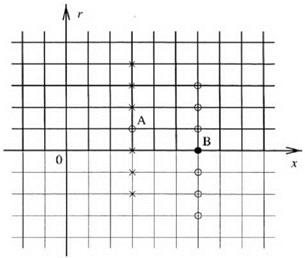
Figure 12.12. Extension of the computational domain, the upper part of the x — r plane, to the nonphysical lower half plane.
points near the axis (but not on the axis such as point A) may be extended into the negative r half-plane as shown. For the points on the axis, such as point B, they will not be calculated by the time marching DRP scheme. They are to be found, after the values at all the other points have been updated to a new time level, by symmetric interpolation. A 7-point interpolation stencil for point B is shown in Figure 12.12.


