Artificial Selective Damping

Artificial selective damping is added to the time marching DRP scheme to eliminate spurious short waves and to prevent the occurrence of numerical instability. The damping stencil with a damping curve of half-width 0.2n is used for background damping. Near the solid walls or the outer boundaries where a 7-point stencil does not fit, a 5- or 3-point stencil as provided in Section 7.4 is used instead. For general background damping, an inverse mesh Reynolds number of 0.05 is used everywhere. Along walls and mesh-change interfaces, additional damping is included. The added damping has an inverse mesh Reynolds number distribution in the form of a Gaussian function with the maximum value at the wall or interface and a half-width of 4 mesh points as in the first example. On the wall, the maximum value of R^1 is set equal to 0.15. The corresponding value at a mesh-size-change interface is 0.3. There are three external corners at the cavity opening. They are probably sites at which short spurious waves are generated. To prevent numerical instability from developing at these points, additional artificial selective damping is imposed. Again, a half-width of 4 mesh point Gaussian distribution of the inverse mesh Reynolds number centered at each of these points is used. The maximum value of R^1 at these points is set equal to 0.35. By implementing artificial selective damping distribution as described, no numerical instability nor excessive short spurious waves have been found in all the computations.

12.4.2.2 Numerical Results

To start the computation, the time-independent boundary layer solution without the cavity is used as the initial condition. The solution is time-marched until a time periodic state is reached.

The characteristic features of the flow in the vicinity of the cavity opening and the acoustic field are found by examining the instantaneous vorticity, steamlines, and pressure contours. Figure 12.16 shows a plot of the instantaneous vorticity contours for the case U = 50.9 m/s and 5 = 2.0 mm. As can easily be seen, vortices are

Figure 12.16. Instantaneous vorticity contours showing the shedding of small vortices at the trailing edge of the cavity. U = 50.9 m/s, S = 2 mm.

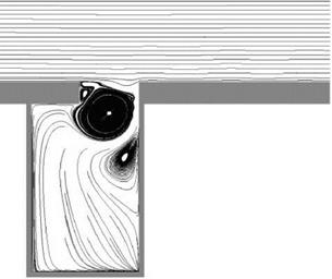
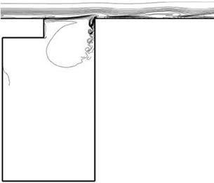shed periodically at the trailing edge of the cavity. Some shed vortices move inside the cavity. Other vortices are shed into the flow outside. The shed vortices outside are convected downstream by the boundary layer flow. These convected vortices are clearly shown in the pressure contour plot of Figure 12.17. They form the low- pressure centers. These vortices persist over a rather long distance and are eventually dissipated by viscosity. Figure 12.18 shows the instantaneous streamline pattern. It is seen that the flow at the mouth of the cavity is completely dominated by a single large vortex. Below the large vortex, another vortex of opposite rotation often exists. The position of this vortex changes from time to time and does not always attach to the cavity wall. The near-field pressure contour pattern is shown in Figure 12.19. This pattern is the same as that of a monopole acoustic source in a low subsonic stream. That the noise source is a monopole, and not a dipole, is consistent with the model of Tam and Block (1978). The sound is generated by flow impinging periodically at the trailing edge of the cavity.

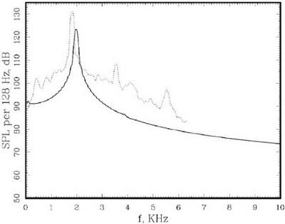
Experiments indicate that cavity resonance may consist of a single tone or mul­tiple tones. The number of tones occured depend on the flow conditions and the cavity geometry. Figure 12.20 shows the noise spectrum measured at the center of the left wall of the cavity at U = 50.9 m/s, S = 2 mm. The spectrum consists of a single tone at 1.99 kHz.

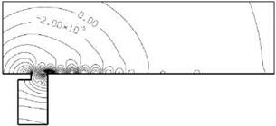Figure 12.17. Near-field pressure con­tours showing the convection of shed vortices along the outside wall. U = 50.9 m/s, S = 2 mm.

Figure 12.18. Instantaneous streamline pattern. U = 50.9 m/s, S = 2 mm.

Shown in Figure 12.20 also is the spectrum measured experimentally by Hender­son (2000). There is good agreement between the tone frequency of the numerical simulation and that of the physical experiment. In the experiment, the boundary layer is turbulent; therefore, it is not expected that there would be good agreement in the tone intensity. Figure 12.21 shows the noise spectrum at the lower speed U = 26.8 m/s and S = 1 mm. In this case, there are two tones. One is at a frequency of 1.32 kHz and the other at 2.0 kHz. This is in fair agreement with the experimentally measured spectrum. Again, the tone frequencies are reasonably well reproduced in the numerical simulation, but the tone intensities are different. Figures 12.20 and 12.21 together suggest that as the flow velocity increases, one of the tones disappears. The strength of the remaining tone intensifies with flow speed.