Our heavyweight helicopter equal in the world does not have
In Rostov started production of the most load-lifting rotary-wing car The Russian holding «Helicopt[...]

Everything about aircrafts and helicopters. News and events in aviation worldwide. Civil, transportation, military helicopters and airplanes.

Everything about aircrafts and helicopters. News and events in aviation worldwide. Civil, transportation, military helicopters and airplanes.

Everything about aircrafts and helicopters. News and events in aviation worldwide. Civil, transportation, military helicopters and airplanes.

Everything about aircrafts and helicopters. News and events in aviation worldwide. Civil, transportation, military helicopters and airplanes.


The power-thrust relationship for level flight was derived in Chapter 5 and is given in idealized form in Equation 5.70, or with empirical constants incorporated in Equation 5.71. Generally we assume the latter form to be the more suitable for practical use and indeed to be adequate for most preliminary performance calculation. The equation shows the power coefficient to be the linear sum of separate terms representing, respectively, the induced power (rotor lift dependent), profile power (blade section drag dependent) and parasite power (fuselage drag dependent). It is in effect an energy equation, in which each term represents a separately identifiable sink of energy, and might have been calculated directly as such. In dimensional terms we have:
in which VT is the rotor tip speed, V the forward flight speed and f the fuselage-equivalent flat plate area, defined in Equation 5.88. The induced velocity Vi is given according to momentum theory by Equation 5.3; however, if we simplify the situation by assuming the rotor disc tilt is very small, Equation 5.3 can be rewritten as:
![]() T 1
T 1
Vi = 2pA ffiTVf
where VZ is neglected as small order compared with Vi and VX becomes V. The solution of (7.10) is given by:
Allowances should be added for tail rotor power and power to transmission and accessories: collecting these together in a miscellaneous item, the total is perhaps 15% of P at V = 0
|
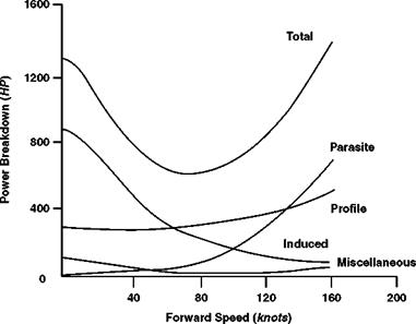
Figure 7.3 Typical power breakdown for forward level flight |
(Section 7.2) and half this, say 8%, at high speed. Otherwise, if the evidence is available, the items may be assessed separately. The thrust T may be assumed equal to the aircraft weight W for all forward speeds above 5 m/s (10 knots) although at the highest speeds, the fuselage drag needs careful attention.
A typical breakdown of the total power as a function of flight speed is shown in Figure 7.3.
Induced power dominates the hover but makes only a small contribution in the upper half of the speed range. Profile power rises only slowly with speed unless and until the compressibility drag rise begins to be shown at high speed. Parasite power, zero in the hover, increases as V3 and is the largest component at high speed, contributing about half the total. As a result of these variations the total power has a typical ‘bucket’ shape, high in the hover, falling to a minimum at moderate speed and rising rapidly at high speed to levels above the hover value. Except at high speed, therefore, the helicopter uses less power in forward flight than in hover.
Charts are a useful aid for rapid performance calculation. If power is expressed as P/d, where d is the relative air density at altitude, a power carpet can be constructed giving the variation of P/d with W/d and V. Figures 7.4a and b show an example, in which for convenience the carpet is presented in two parts, covering the low – and high-speed ranges. When weight, speed and density are known, the power required for level flight is read off directly.
The above is a relatively simple analysis of helicopter performance. The Appendix contains a fuller description of power prediction, the associated fuel consumption and mission analysis.