Lateral motion

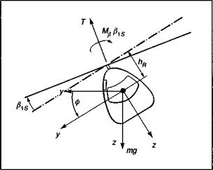
We consider a simple model of a helicopter being flown along a prescribed flight path in two-dimensional, horizontal flight (Fig. 5.7). The key points can be made with the most elementary simulation of the helicopter flight dynamics (i. e., quasi-steady rotor dynamics). It is assumed that the pilot is maintaining height and balance with collective and pedals, respectively. The equation for the rolling motion is given in terms of the lateral flapping Ps:

IxxФ = ~Mp Pis (5.35)

Fig. 5.7 Helicopter force balance in simple lateral manoeuvre

where Mp is the rolling moment per unit flapping given by

Mp = (+ hRT) (5.36)

The rotor thrust T varies during the manoeuvre to maintain horizontal flight. As de­scribed in Chapter 3, the hub stiffness Kp can be written in terms of the flap frequency ratio Xp, flap moment of inertia Ip and rotorspeed Й, in the form

Kp = (k2p – l) (5.37)

The equations of force balance in earth axes can be written as

T cos (ф – Pis) = mg (5.38)

T sin (ф – Pis) = my (5.39)

where y(t) is the lateral flight path displacement. Combining eqns 5.35, 5.38 and 5.39, and assuming small roll and lateral flapping angles (including constant rotor thrust), we obtain the second-order equation for the roll angle ф

Where v is the normalized sideforce (i. e., lateral acceleration) given in linearized form by

v = y/g (5.4l)

and the ‘natural’ frequency оц is related to the rotor moment coefficient by the expres­sion

(5.42)

The rotor and fuselage roll time constants are given in terms of more fundamental rotor parameters, the rotor Lock number (y) and the roll damping derivative (Lp)

The reader should note that the assumption of constant frequency оф implies that the thrust changes are small compared with the hub component of the rotor moment. The frequency Оф is equal to the natural frequency of the roll-regressive flap mode

discussed in Chapters 2 and 4.

Equation 5.40 holds for general small amplitude lateral manoeuvres and can be used to estimate the rotor forces and moments, hence control activity, required to fly a manoeuvre characterized by the lateral flight path y(t). This represents a simple case of so-called inverse simulation (Ref. 5.13), whereby the flight path is prescribed and the equations of motion solved for the loads and controls. A significant difference between rotary and fixed-wing aircraft modelled in this way is that the inertia term

in eqn 5.40 vanishes for fixed-wing aircraft, with the sideforce then being simply proportional to the roll angle. For helicopters, the loose coupling between rotor and fuselage leads to the presence of a mode, with dynamics described by eqn 5.40, with frequency шф, representing an oscillation of the aircraft relative to the rotor, while the rotor maintains the prescribed orientation in space. We have already seen evidence of a similar mode in the previous analysis of constrained vertical motion. Oscillations of the fuselage in this mode, therefore, have no effect on the flight path of the aircraft. It should be noted that this ‘mode’ is not a feature of unconstrained flight, where the two natural modes are a roll subsidence (magnitude Lp) and a neutral mode (magnitude 0), representing the indifference of the aircraft dynamics to heading or lateral position. The degree of excitation of the ‘new’ free mode depends upon the frequency content of the flight path excursions and hence the sideforce v. For example, when the prescribed flight paths are genuinely orthogonal to the free oscillation (i. e., combinations of sine waves), then the response will be uncontaminated by the free oscillation. In practice, slalom-type manoeuvres, while similar in character to sine waves, can have significantly different load requirements at the turning points, and the scope for excitation of the free oscillation is potentially high. A further important point to note about the character of the solution to eqn 5.40 is that as the frequency of the flight path approaches the natural frequency шф, the roll angle approaches a ‘resonance’ condition. To understand what happens in practice, we must look at the equation for ‘forward’ rather than ‘inverse’ simulation. This can be written in terms of the lateral cyclic control input Qc forcing the flight path sideforce v, in the approximate form

The derivation of this equation depends on the assumption that the rotor responds to control action and fuselage angular rate in a quasi-steady manner, taking up a new disc tilt instantaneously. In reality the rotor responds with a time constant equal to (16/y Й), but for the purposes of the present argument this delay will be neglected. The presence of the control acceleration term on the right-hand side of eqn 5.44 is crucial to what happens close to the natural frequency. In the limit, when the input frequency is at the natural frequency, the flight path response is zero due to the cancelling of the control terms, hence the implication of the theoretical artefact, in eqn 5.40, that the roll angle would grow unbounded at that frequency. As the pilot moves his stick at the critical frequency, the rotor disc remains horizontal and the fuselage wobbles beneath. We found a similar effect for longitudinal motion. For cyclic control inputs at slightly lower frequencies, the sideforces are still very small and large control displacements are required to generate the turning moments. Stick movements at frequencies slightly higher than шф produce small forces of the opposite sign, acting in the wrong direction. Hence, despite intense stick activity the pilot may not be able to fly the desired track. The difference between what the pilot can do and what he is trying to do increases sharply with the severity of the desired manoeuvre, and the upper limit of what can usefully or safely be accomplished, in terms of task ‘bandwidth’, is determined by the frequency шф. For current helicopters, the natural frequency шф varies from 6 rad/s for low hinge offset, slowly rotating rotors, to 12 rad/s for hingeless rotors with higher rotor speeds.

Two questions arise out of the above simple analysis. First, as the severity of the task increases, what influences the cut-off frequency beyond which control activity becomes unreasonably high and hence can this cut-off frequency be predicted? Second, how does the pilot cope with the unconstrained oscillations, if indeed they manifest themselves in practice. A useful parameter in the context of the first question is the ratio of aircraft to task natural frequencies. The task natural frequency can, in general, be derived from a frequency analysis of the flight path variation, but for simple slalom manoeuvres the value is approximately related to the inverse of the task time. It is suggested in Ref. 5.12 that a meaningful upper limit to task frequency can be written in the form

^ > 2nv (5.45)

&t

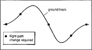
where nv is the number of flight path changes required in a given task. A two-sided slalom, for example, as illustrated in Fig. 5.8, contains five such distinct changes; hence at a minimum, for slalom manoeuvres

Ют

-т> 10 (5.46)

This suggests that a pilot flying a reasonably agile aircraft, with юф = 10 rad/s, could be expected to experience control problems when trying to fly a two-sided slalom in less than about 6 s. A pilot flying a less agile aircraft (юф = 7 rad/s) might experience similar control problems in a 9-s slalom. This 50% increase in usable performance for an agile helicopter clearly has very important implications for military and some civil operations.

Figures 5.9(a)-(c) show results from an inverse simulation of Helisim Lynx fitted with different rotor types flying a slalom mission task element (Ref. 5.12). Three rotor configurations are shown on the figures corresponding to юф = 11.8 (standard Lynx), юф = 7.5 (articulated) and юф = 4.5 (teetering). The aspect ratio of the slalom, defined as the overall width to length, is 0.077, the maximum value achievable by the teetering rotor configuration before the lateral cyclic reaches the control limits; the flight speed is 60 knots. Figures 5.9(a) and (b) show comparisons of the roll attitude and rate responses respectively. The attitude changes, not surprisingly, are very similar for the three cases,

Fig. 5.8 Flight path changes in a slalom manoeuvre (Ref. 5.12)

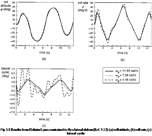
as are the rates, although we can now perceive the presence of higher frequency motion in the signal for the teetering and articulated rotors. For the teetering rotor, roll rate peaks some 10 – 20% higher than required with the hingeless rotor can be observed – entirely a result of the component of the free mode in the aircraft response. Figure 5.9(c) illustrates the lateral cyclic required to fly the 0.077 slalom, the limiting aspect ratio for the teetering configuration. The extent of the excitation of the roll oscillation for the different cases, and hence the higher frequency ‘stabilization’ control inputs, is shown clearly in the time histories of lateral cyclic. The difference between the three rotor configurations is now very striking. The Lynx, with its standard hingeless rotor, requires 30% of maximum control throw, while the articulated rotor requires slightly more at about 35%.

In Ref. 5.12, the above analysis is extended to examine pilot workload metrics based on control activity. The premise is that the conflict between guidance and stabi­lization is a primary source of workload for pilots as they attempt to fly manoeuvres beyond the critical aircraft/task bandwidth ratio. Both time and frequency domain workload metrics are discussed in Ref. 5.12, and correlation between inverse simu­lation and Lynx flight test results is shown to be good; the limiting slalom for both cases was about 0.11. This line of research to determine reliable workload metrics for

predicting critical flying qualities boundaries is, in many ways, still quite formative, and detailed coverage, in this book, of the current status of the various approaches is therefore considered to be inappropriate.

The topic of stability under constraint is an important one in flight dynamics, and the examples described in this section have illustrated how relatively simple anal­ysis, made possible by certain sensible approximations, can sometimes expose the physical nature of a stability boundary. This appears fortuitous but there is actually a deeper underlying reason why these simple models work so well in predicting prob­lems. Generally, the pilot will fly a helicopter using a broad range of control inputs, in terms of both frequency and amplitude, to accomplish a task, often adopting a control strategy that appears unnecessarily complex. There is some evidence that this strat­egy is important for the pilot to maintain a required level of attention to the flying task, and hence, paradoxically, plentiful spare capacity for coping with emergencies. Continuous exercise of a wide repertoire of control strategies is therefore a sign of a healthy situation with the pilot adopting low to moderate levels of workload to stay in command. A pilot experiencing stability problems, particularly those that are self­induced, will typically concentrate more and more of his or her effort in a narrow frequency range as he or she becomes locked into what is effectively a man-machine limit cycle. Again paradoxically, these very structured patterns of activity in pilot con­trol activity are usually a sign that handling qualities are deteriorating and workload is increasing.