Optimized Multidimensional Interpolation

The idea and methodology of optimized multidimensional interpolation will be considered first. Numerical examples will be given later. For simplicity, only two­dimensional interpolation is discussed in detail. The generalization to three dimen­sions is fairly straightforward.

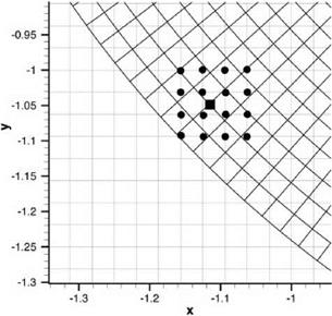Figure 13.5. Interpolation from a Carte­sian grid to a polar grid using a 16-point stencil. Ax = Ay = Ar = 1/32.

Figure 13.6. A 16-point irregular inter­polation stencil.

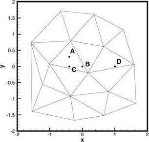The development of optimized multidimensional interpolation is, in many respects, similar to that in one dimension. Consider an interpolation stencil in a computational domain as shown in Figure 13.6. Without loss of generality, the inter­polation is considered for implementation in the x – y plane. However, x and y may be a set of curvilinear coordinates in the physical domain. For interpolation purposes, the values of a function f(x, y) are given at the stencil points (x, y), j = 1,2,…, N for an N-point stencil. The objective is to estimate the value f(xo, yo) at a general point P at (xo, yo). By definition of interpolation (not extrapolation), the point P lies within the boundary of the stencil as defined by Figure 13.6. Let dj be the distance between neighboring points of the stencil. A useful length scale is

1 K

A = – J2 dj. (13.3)

j=1

where K is the number of links between stencil points.

The most general interpolation formula in two dimensions has the following form:

N

f (xo. Уо) = Y^ Sjf (xj > yj )• (13.4)

j=1

Different interpolation methods determine the coefficient Sj in different ways.

It will be assumed that the function f(x, y) to be interpolated has a Fourier inverse transform, such that

TO TO

f(X. y) = ft«.e)e»+ey>d«de. (13’5)

-TO – TO

where (а, в) are the wave numbers in the x and y directions, respectively.

Let A(a, в) = | f (а, в)| and ф(а, в) = arg[f (а, в)], Eq. (13.5) maybe rewritten

w w

f {x-» = f ІА(а-в)Є’‘х+п^а (136)

This equation may be interpreted in the sense that f(x, y) is made up of a superposition of simple waves exp[i(ax + by + ф(а, b))] with amplitude A(a, в). It is useful to define the local interpolation error, Elocal, for wave number (а, в) as the absolute value of the difference between the left and right side of Eq. (13.4) when f(x, y) is replaced by the simple wave as follows:

Here all simple waves are assumed to have unit amplitude; i. e., А(а, в) = 1.0. It is easy to find as follows:

N

■ j = 1

The total error, E, over the region – к < аД, вД < к, in wave number space is

obtained by integrating Efocal of Eq. (13.8) over this region, i. e.,

When the function to be interpolated is a constant, which corresponds to setting а = в = 0 in Eq. (13.7), it is reasonable to require the local interpolation error to be zero. By Eq. (13.8), this requirement leads to

N

ES; -1 = 0

j=1

It is now proposed that the interpolation coefficients, Sj (j = 1, 2,…, N) be chosen such that E2 is a minimum subjected to constraint (13.10). This can readily be done by using the method of the Lagrange multiplier. Let

where k is the Lagrange multiplier. The conditions for L to be a minimum are

dL = 0, dL = 0, j = 1,2,…,n. (13.12)

It is easy to find that the condition dL/дSj = 0 yields

where Re{} is the real part of {}. Similarly it is easy to find that 9L/дк leads to

N

ESj -1 = 0

which is constraint (13.10).

Eqs. (13.13) and (13.14) form a linear matrix system of (N + 1) unknowns for Sj (j = 1,2,…, N) and к. It turns out that all the integrals of Eq. (13.13) can be evaluated in closed form. This allows the matrix elements to be written out explicitly. The values of Sj may be found by solving the matrix system as follows:

AS = b, (13.15)

where vector ST = (S1 S2 S3 … SN к). Note: Superscript T denotes the transpose. The elements of the coefficient matrix A and vector b are given by

Note: In the case Xj = Xk and/or yj = yk or Xj = X0 or yj = y0 the limit forms of these formulas are to be used. Computationally, the limit forms are used wherever |Xj – xk| < c or |yj – yk| < c. This is discussed in Appendix 13A at the end of of this chapter.

It is useful to point out that Ajk depends on A and К as well as the coordinates of the stencil points only. The coordinates of the point to be interpolated to, (x0, y0), appears only in bj. Thus, if many values of f are to be interpolated using the same stencil, A and A-1 need only be computed once.

For error estimate purposes, the following symmetry properties of the local error, given by Eq. (13.8), can easily be derived.

£local (а, в) = Elocal (-a> – У Elocal (-а, в) = Elocal (a> -в) .

Thus, once S/s are found, Elocal can be calculated by formula (13.8). Upon invoking Eqs. (13.22) and (13.23), it is sufficient to examine Elocal(a, в) over the upper half of the aA – в A plane for – п < а А, в A < п.