Sliding Interface Problems

13.4.1 Sliding Interface Problem in Two Dimensions

Aircraft engine noise is a significant environmental and certification issue. Noise generated by the fan rotor wake impinging on the stator is an important noise com­ponent at both takeoff and landing. In the Second CAA Workshop on Benchmark

Figure 13.17. Zero pressure contours at the beginning of a cycle. Pressure pat­tern formed by the scattering of a plane wave by a cylinder. Wavelength equal to quarter diameter of cylinder.

Problems, a simplified model of this noise mechanism was proposed as a benchmark problem. One important feature of the problem is a sliding interface imitating the relative motion between a fan blade fixed computation domain and a stator blade fixed computation domain. Here, a less demanding sliding interface problem is con­sidered. It will be shown that the use of an optimized interpolation scheme and overset grids method yields accurate numerical results.

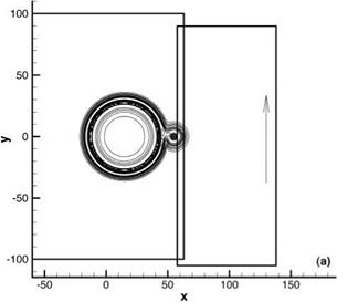
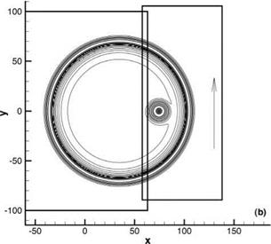
Figure 13.19 shows two computation planes with six columns of overlapping meshes. The left computation plane is stationary. The right computation plane moves upward at a velocity of vg. The sliding interface is the line at the center of the overlapping meshes. (x1, y1) will be used to denote the coordinates of a point in the stationary computation plane on the left, and (x2, y2) will be used to denote the coordinates of a point in the moving computation plane on the right. The relationships between the two coordinate systems are x2 = x1, y2 = y1 – vgt.

For computation purposes, square meshes are used in each computation plane, i. e., Ax1 = Ayx, Ax2 = Ay2 = 0.78Ax1. However, the mesh sizes are not the same in the two computation grids. Dimensionless variables with Ax1 as length scale, a0 (the speed of sound) as the velocity scale, Ax1/a0 as the time scale, p0 (mean flow density) as the density scale, and p0a2 as the pressure scale are used. It will be assumed that there is a uniform mean flow at 0.5 Mach number in the x direction over the entire computation domain. The x direction is the horizontal direction in Figure 13.19. The sliding interface is at x = 60.

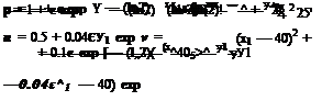
The governing equations are the Euler equations. In the stationary computation plane, they are given by Eq. (13.1) with x replaced by x1 and y replaced by y1. In the moving computation plane, the governing equations, with respect to a grid fixed frame of reference, are:

d v d v 9 v 1 9 p

— + u— + (v — vg)— +—————- = 0

dt 9×2 g dy2 p dy2

At time equal to zero, a pressure pulse centered at x1 = y1 = 0 is released. At the same time, a vorticity pulse and an entropy pulse centered at x1 = 40, y1 = 0 are released. Mathematically, the initial conditions at t = 0 are as follows:

where c = 0.005 and y = 1.4. In the course of time, the acoustic, the vorticity, and the entropy pulse will all be propagating or convected downstream. They will all reach the sliding interface at nearly the same time. They will then move across the sliding interface into the moving grid farther downstream. The exact solution of this problem was given in Section 6.4.

In the computation, the 7-point stencil DRP scheme is again used. For points on the stationary grid, the unknowns on every grid point including those on the sliding interface are determined at every time step by solving Eq. (13.1). Similarly, for points on the moving grid, the unknowns on every grid point including those on the sliding interface are updated according to Eq. (13.43). The unknowns of the three extra columns of grid points extending beyond the sliding interface are not calculated by the 7-point stencil DRP scheme. They are found by optimized interpolation using a 16-point stencil from the values of the variables on the other grid. In this way, information of the solution is passed between the two computation grids.

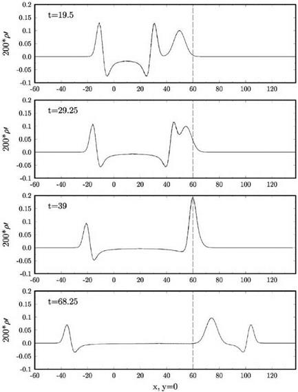
Figures 13.19a-13.19c show the computed density contours associated with the acoustic and entropy pulses at time t = 5.6, 44.9, and 73.0. In this computation vg is set equal to 0.4. Also plotted in these figures are contours of the exact solution in dashed lines. Because the difference between the computed and the exact solution is small, the dashed lines may not be easily detected. In Figures 13.19a, the two pulses are in the stationary grid. Figures 13.19b shows that the acoustic pulse, moving downstream at three times the velocity of the entropy pulse, catches up with the entropy pulse right at the sliding interface. Figures 13.19c shows that the entropy pulse has now been convected past the sliding interface onto the moving grid. At this time, the acoustic pulse has already propagated further downstream. Figure 13.20 shows the computed and the exact density waveform along the x-axis at four different times. The sliding interface is located at x = 60. It is clear from these figures that

Figure 13.20. Spatial distribution of density perturbation p’ = p — 1 associated with an acoustic and an entropy pulse propagating across a sliding interface located at x = 60. Dashed line is the exact solution.

the treatment of a sliding interface using optimized interpolation is effective and accurate.

Figures 13.21a and 13.21b show the computed and the exact fluid velocity exclud­ing the mean flow, (w/2 + v/2)1/2, contours of the acoustic and vorticity pulses as they propagate through the sliding interface. Again, the difference between the computed and exact contours, being less than the thickness of the contour lines, is difficult to detect. Figure 13.22 shows the waveform along the x-axis at four instances of time. At t = 29.25 to t = 39, the two pulses merge and propagate across the sliding inter­face together. At time t = 68.25, the acoustic pulse has passed through the entropy

Figure 13.21. Contours of fluid velocity (и’2 + v’2)1/2 associated with the trans­mission of an acoustic and a vorticity pulse across a sliding interface. Dashed lines are the exact solution. (a) t = 28.1. (b) t = 67.3.

pulse and the two pulses are now separated. The computed waveforms are in good agreement with the exact solution.

In this computation, the moving grid moves at a subsonic velocity. In a similar computation the same results are recovered when the moving grid slides past the stationary grid at a supersonic velocity.