Our heavyweight helicopter equal in the world does not have
In Rostov started production of the most load-lifting rotary-wing car The Russian holding «Helicopt[...]

Everything about aircrafts and helicopters. News and events in aviation worldwide. Civil, transportation, military helicopters and airplanes.

Everything about aircrafts and helicopters. News and events in aviation worldwide. Civil, transportation, military helicopters and airplanes.

Everything about aircrafts and helicopters. News and events in aviation worldwide. Civil, transportation, military helicopters and airplanes.

Everything about aircrafts and helicopters. News and events in aviation worldwide. Civil, transportation, military helicopters and airplanes.


In the UK Airworthiness Defence Standard (Ref. 5.45), turbulence intensity is characterized by four bands: light (0-3 ft/s), moderate (3-6 ft/s), severe (6-12 ft/s) and extreme (12-24 ft/s). A statistical approach to turbulence refers to the probability of equalling or exceeding given intensities at defined heights above different kinds of terrain. A second important property of turbulence is the relationship between the intensity and the spatial or temporal scale or duration, which also varies with height above terrain. Such a classification has obvious attractions for design and certification purposes, and the extensions of fixed-wing methods to helicopters are generally applicable at operating heights above about 200 ft. Below this height, the dearth of measurements of three-dimensional atmospheric disturbances means that the characterization of turbulence is less well understood, with the distinct exception of airflow around man-made constructions (Ref. 5.46). For the purposes of this discussion, we circumvent this dearth of knowledge and concern ourselves only with the general modelling issues rather than specific cases, but it is important to note that extensions of results from fixed-wing studies may well not apply to helicopters. Another area where this read-across has to be reinterpreted is the treatment of turbulence scale length. In fixed-wing work a common approximation assumes a ‘frozen-field’ of disturbances, such that the scale length and duration are related directly through the forward speed of the aircraft. For helicopters in hover or flying through winds at low speed, this approach is clearly not valid and it is more appropriate to consider the aircraft flying through (or hovering in) a steady wind with the turbulence superimposed.
The most common form of turbulence model involves the decomposition of the velocity into frequency components, where the rms of the aircraft response can be related to the rms intensity of the turbulence. In Ref. 5.45, this power spectral density (PSD) method is recommended for investigations of general handling qualities in continuous turbulence. The PSD contains information about the excitation energy within the atmosphere as a function of frequency (or spatial wavelength), and several models exist based on measurements of real turbulence. For example, the von Karman PSD of the vertical component of turbulence takes the form (Refs 5.47, 5.48)
where the wavenumber v = frequency/airspeed, L is the turbulence scale and a is the rms of the intensity. The von Karman method assumes that the disturbance has Gaussian properties and the extensive theory of stationary random processes can be brought to bear when considering the response of an aircraft as a linear system. This is clearly a strength of the approach but it also reveals a weakness. A significant shortcoming of the basic PSD approach is its inability to model any detailed structure in the disturbance. Large peaks and intermittent features are smoothed over as the amplitude and phase characteristics are assumed to be uniformly distributed across the spectrum. Any phase correlations in the turbulence record are lost in the PSD process, hence removing the capability of sinusoidal components reinforcing one another. Atmospheric disturbances with highly structured character, corresponding for example to shear layers exhibiting sharp velocity gradients, are clearly important for helicopter applications in the wake of hills and structures, and a different form of modelling is required in these cases.
|
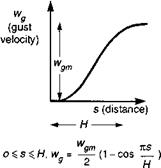
Fig. 5.33 Elemental ramp gust used in the statistical discrete gust approach |
The statistical discrete gust (SDG) approach to turbulence modelling was developed by Jones at DRA (RAE) for fixed-wing applications (Refs 5.49-5.51), essentially to cater for more structured disturbances, and appears to be ideally suited for low – level helicopter applications. In Ref. 5.45, the SDG method is recommended for the assessment of helicopter response to, and recovery from, large disturbances. The basis of the SDG approach is an elemental ramp gust (Fig. 5.33) with gradient distance (scale) H and gust amplitude (intensity) Wg. A non-Gaussian turbulence record can be reconstituted as an aggregate of discrete gusts of different shapes and sizes; different elemental shapes, with self-similar characteristics (Ref. 5.49), can be used for different forms of turbulence. One of the properties of turbulence, correctly modelled by the PSD approach, and that the SDG method must preserve, is the shape of the PSD itself which appears to fit measured data well. This so-called energy constraint (Ref. 5.50) is satisfied by the self-similar relationship between the gust amplitude and length in the aggregate used to build the equivalent SDG model. For example, with the VK spectrum, the relationship takes the form wg a H1/3 for gusts with length small compared with the reference spectral scale L.
Where the PSD approach adopts frequency-domain, linear analysis, the SDG approach is essentially a time-domain, nonlinear technique. Since the early development of the SDG method, a theory of general transient signal analysis has been developed, providing a rational framework for its use. The basis of this analysis is the so-called ‘Wavelet’ transform, akin to the Fourier transform, but returning a new time-domain function of scale and intensity (Ref. 5.51). The SDG elements can now be interpreted as a particular class of wavelet, and a turbulence time history can be decomposed into a combination of wavelets adopting the so-called adaptive wavelet analysis (Ref. 5.48). These new techniques provide considerably more flexibility in the modelling of structured turbulence and should find regular use in helicopter response analysis.
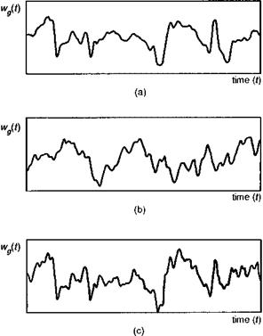
To close this brief review of turbulence modelling, Fig. 5.34 illustrates the comparison between two forms of turbulence record reconstruction (Ref. 5.48). The measurements exhibit features common to real atmospheric disturbances – sharp velocity gradients associated with shear layers and periods of relative quiescence (Fig. 5.34(a)). Figure 5.34(b) shows the turbulence reconstructed using measured amplitude components with random phase components from the PSD model. From a PSD perspective, the information in Fig. 5.34(b) is identical to the measurements, but it can be seen that all structured features in the measurements have apparently disappeared in the
|
Fig. 5.34 Influence of Fourier amplitude and phase on the structure of atmospheric turbulence: (a) measured atmospheric turbulence; (b) reconstruction using measured amplitude components; (c) reconstruction using measured phase components |
reconstruction process. Figure 5.34(c), on the other hand, has been reconstructed using the measured phase components with random amplitude components from the PSD model. The structure has been preserved in this process, clear evidence of the nonGaussian characteristics of these turbulence measurements, where the real phase correlation has preserved the reinforcement of energy present in the concentrated events. These structured features of turbulence are important for helicopter work. They occur in the nap-of-the-earth and close to oil rigs and ships. Their scales can also be quite small and, at low helicopter speeds, scale lengths as small as the rotor radius can influence ride and handling.