Fuzzy Kalman Filter for State Estimation

It is essential to obtain accurate estimation of target states (position, velocity, and acceleration) from the noisy measurements originating from single or multiple sensors. KF is a suitable algorithm for such applications. In the case of multiple sources, either single KF can be used by fusing the measurements at data level or one can use state vector fusion. The accuracy of estimated/fused states depends on (1) how precisely the target and measurement models are known and (2) tuning param­eters such as process noise covariance matrix “Q” and measurement noise covar­iance matrix ‘‘R,’’ which basically decide the bandwidth of the filter. In many situations, either mathematical models are not known accurately or are difficult to model. In practice, modeling errors are partially compensated by tuning Q, using trial

TABLE 9.14 Estimates by Adaptive Neuro-Fuzzy Inference System Estimated Values Parameters True Values No Noise SNR = 10 a 1 0.9999 0.9999 b 2 2.0000 2.0000 c 1 0.9999 0.9999

and error or some heuristic approach. A fuzzy Kalman filter (FKF) is found suitable in such cases and it is investigated here. The performances of KF and FKF are compared with adaptive Kalman filter (AKF) in which the process noise covariance Q is computed online using the sliding window method.

FL is a multivalue logic (Chapter 2) used to model any event or condition that is not precisely defined or is unknown. In the FL-based system we use (1) membership function (fuzzification)—it converts the I/O crisp values to corre­sponding membership grades indicating its belongingness to respective fuzzy set; (2) rule base consisting of IF-THEN rules; (3) fuzzy implications used to map the fuzzified input to an appropriate fuzzified output; (4) aggregation used to combine the output fuzzy sets (single output fuzzy set for every rule fired) to single fuzzy set, and (5) defuzzification to convert the aggregated output fuzzy set from its fuzzified values to equivalent crisp values (Figure 2.20). In a KF, since the innovation sequence is the difference between sensor measurement and predicted value (based on the filter’s internal model), this mismatch can be used to perform the required adaptation using fuzzy logic rules. The advantages derived from the use of the fuzzy technique are the simplicity of the approach and the possibility of accommodating the heuristic knowledge about the phenomenon. This aspect is accommodated in Equation 9.44 as given by

X(k + 1/k + 1) = X(k + 1 /k) + KC(k + 1) (9.87)

Here, C(k + 1) is the fuzzy correlation variable (FCV) [36] and is a nonlinear function of the innovations vector e. It is assumed that target motion in each axis is independent. FCV consists of two inputs (i. e., ex and Єх) and single output cx(k + 1), where Єх is computed by

Here, T is the sampling time interval in seconds. In any FIS, fuzzy implication provides mapping between input and output fuzzy sets. Basically, a fuzzy IF-THEN rule is interpreted as a fuzzy implication. The antecedent membership functions would define the fuzzy values for inputs ex and ex. The labels used in linguistic variables to define membership functions are LN (large negative), MN (medium negative), SN (small negative), ZE (zero error), SP (small positive), MP (medium positive), and LP (large positive). The rules for the inference in FIS are created based on past experiences and intuitions. For example, one such rule is

If ex is LP and ex is LP then cx is LP (9.89)

This rule is created based on the fact that having ex and ex with large positive values indicates an increase in innovation sequence at a faster rate. The future value of ex (and therefore ex) can be reduced by increasing the present value of cx (a function of« Z — HX) with a large magnitude. Table 9.15 summarizes the 49 rules [36] used to implement FCV. Output cx at any instant of time can be computed using the inputs

ex and ex, input membership functions, rules mentioned in Table 9.15, fuzzy infer­ence engine, aggregator, and defuzzification.

The properties of FIS used in the present work are as follows: (1) its type is Mamdani; (2) AND operator is Min; (3) OR operator is Max; (4) implication used is Min; (5) Aggregation used is Max; and (6) the defuzzification used is Centroid (Figure 2.20).

Example 9.3: Target Tracking

The relevant MATLAB programs are “ExampSolSW/Example 9.3FKTT49Rules, 9.3FKTT4Rules, 9.3AKF.’’ The target data in x, y-direction are generated using the constant acceleration model with process noise increment [37]. With sampling interval T — 0.1 s, a total of N — 100 scans are generated. The data simulation proceeds with the following assumed parameter values and equations: (1) initial states of target x, x, x are 0 m, 100 m/s, and 0 m/s2, respectively, and initial states of y, y, у are 0 m,

— 100 m/s, and —10 m/s2, respectively; and (2) process noise variance Q — 0.0001. The target state equation is X(k + 1) — FX(k) + Gw(k) where, k is the scan number and w is the white Gaussian process noise with zero mean and covariance Q. The measurement equation is Zm(k) — HX(k) + v(k) with H — [1 0 0] and x and v are the measurement noise with zero mean and covariance R — S(s — 10 m). The system matrices are given as

(9.90)

	T3 /6 0 0 1 0 0 ‘	T2/2 0′ 0
T ]	(9.91) (9.92) (9.93)
R =
0

The initial conditions, F, G, H, Q, and R for both the filters are kept the same. The initial state vector X(0/0) is kept close to true initial states. The results for both the filters are compared in terms of true and estimated states and state errors with bounds at every scan number. Every effort was made to tune the KF properly. The same FCV is used for x, y-directions. The performances of both schemes are also compared in terms of RSSPE (root sum square position error) — J(x(k/k) — x(k/k))2 + (y(k/k) — y(k/k))2. Figure 9.13 compares the RSSPE computed using true and estimated states for both the filters. Although the performance of the KF is satisfactory and acceptable, the FKF performs better than the KF. For the same target data (i. e., x – and y-axes), the perform­ance of KF with FKF is compared for two cases: (1) when all the 49 rules are taken into consideration and (2) when only 4 rules are used (Table 9.16).

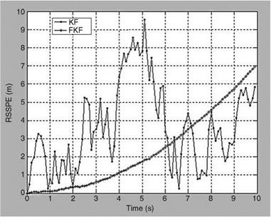Figure 9.14 compares the RSSPE of FKF for these two cases. It is clear that the filter with 49 rules shows better performance than the filter with 4 rules, although the performance with 4 rules is quite acceptable. This indicates that to have a good FKF just a small number of rules is sufficient to obtain continuous and smooth I/O mapping. Too many rules are often unnecessary.