Tracking of Maneuvering Target

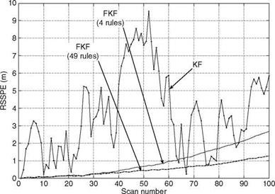
For tracking a maneuvering target, it is essential to redesign the FCV to capture the various possible maneuver modes of the target. Redesigning of FCV involves the following: (1) proper selection of membership functions of inputs and output; (2) tuning of selected membership functions; (3) proper selection of fuzzy operators (e. g., t-norm and s-norm) [38]; and (4) proper selection of fuzzy implication, aggregation, and defuzzification methods. The MATLAB based functions such as “genfis1()” to create initial FCV and “anfis()’’ to tune it are used. These functions require training and check data, which are obtained from true and measured target positions. The target states are generated using a 3DOF kinematic model with process noise acceleration increments, Equations 9.90 through 9.93, and additional arbitrary accelerations. With a sampling interval of 1 s, a total of 150 scans are generated. The data simulation proceeds with the following assumed parameter values: (1) Initial states x, x, x, y, y, y of target are 100, 30, 0, 100, 20, 0, respectively.

(2) Process noise variance Q = 0.1. It is assumed that Qxx = Qyy = Q. (3) Measure­ment noise variance R = 25. It is assumed that Rxx = Ryy = R. It is further assumed that the target has an additional acceleration of (xacc, yacc) at certain scans and an acceleration of (—xacc, — yacc) at certain other scans. Data simulation is carried out using the base state model with process noise vector w (which is a 2 x 1 vector) modified to include additional accelerations at the specified scan points, to induce a specific maneuver as follows:

At the other scan points, the vector w is simply defined by

w(1) = gauss() *vQXX’I w(2) = gauss() *у/0УУ J

The function gauss() uses a central-limit theorem to generate Gaussian random numbers with mean 0 and variance 1. The initial FCV for x-axis is created and tuned using inputs uj, «2, and output oX obtained using the following equations:

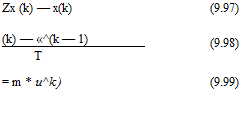
Here, x, zx are true and measured target x-positions, respectively. m is the unknown parameter, which should be properly selected based on maneuver capability of a particular target of interest. For the present case, m = 2 (half of the total simulated points for training and remaining half as a checking data set). The same procedure is followed to obtain tuned-FCV for y-axis. The trained FCV are then plugged into FKF. To generate mild maneuver data, the accelerations are injected at scans 8 (xacc = 6 m/s2 and yacc = —6 m/s2) and 15 (xacc = —6 m/s2 and yacc = 6 m/s2)

only. The performance of FKF is compared with KF and AKF. The equations of AKF are the same as those of KF but with varying process noise covariance Q, estimated online using Maybeck’s method [2]. The equations required to estimate Q are given by

Q(k) = G#[P— — FP+FT ](G#)T (9.100)

P— = K(k)A(k) * (HT)#

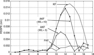
Scan number FIGURE 9.15 RSSPE for KF, FKF, and AKF for tracking of a maneuvering target (Example 9.3).

P+ = P— — K(k)HP — (9.102)

1 k

A(k) = — ]T e(j)e(j)T; k > WL (9.103)

WL j=k-WL+1

Here, # stands for pseudo-inverse, e is the innovation sequence vector, and WL (= 5 for the present case) is the window length. It is important to note that online value of Q can be made available to AKF only from WLth scan, which means that accuracy of Q will depend on its initial guess (for k = 1to WLth — 1 scans) chosen by a filter designer. The AKF exhibited better tracking accuracy, especially during target maneuver, than KF but it had slightly degraded performance compared with FKF. For nonmaneuver­ing phases of target motion, AKF and KF perform almost similarly. During the maneuvering portion, it is found that the magnitude of online Q increases and so the Kalman gain; hence, automatically more weight is assigned to the measurement model, which aids in convergence of the estimated states to true values at a much faster rate than that seen for KF only. A sensitivity study of AKF with respect to different values of WL (5 and 10) was carried out and its performance in terms of RSSPE is compared with KF and FKF (Figure 9.15). It is observed that RSSPE of AKF during the maneuvering phase is high for WL = 10 as compared to WL = 5. This could be due to nonavailability of online Q and with an assumption that its initial guess is not sufficient at a time when actual maneuver starts, i. e., at k = 8.