Aerofoils of Small Aspect Ratio

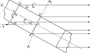
For aerofoils with aspect ratio less than about unity, the agreement between theoretical and experimental lift distribution breaks down. The reason for this breakdown is found to be the consequence of Prandtl’s hypothesis that the free vortex lines leave the trailing edge in the same line as the main stream. This assumption leads to a linear integral equation for the circulation. Let us consider a portion of a flat rectangular aerofoil whose chord c is large compared to the span 2b, as shown in Figure 8.23. Let us take the chord axes with the origin at the center of the rectangle.

The bound vorticity у (x) is assumed to be independent of y, that is to say is constant across a span such as PQ but is variable along the chord. The downwash is also assumed to be independent of y and may therefore be calculated at the center of each span. The main point of the theory developed for aerofoils of small aspect ratio is that the trailing vortices, which leave the tips of each span such as PQ, make an angle в with the chord which is different from a, the incidence, since the trailing vortices follow the fluid

Figure 8.23 A portion of a flat rectangular aerofoil of small aspect ratio.

particles which leave the edges of the aerofoil at angle в will presumably be a function of x. To a first approximation it is assumed to be constant.

8.13.1 The Integral Equation

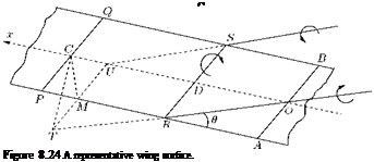
Let us begin with the calculation of the velocity induced at the center C(x, 0, 0) of the span PQ, shown in Figure 8.24.

Consider then the span RS, center D(§, 0, 0). The bound vortex associated with RS is of circulation Y(§) d§ and induces at C a velocity, in the z-direction:

Y (§) d§ .

dwi =————— (cos ZCRS + cos ZCSR) .

4n • CDK +

This gives the downwash due to the whole set of bound vortices as:

This is the velocity induced in the z-direction. If ui is the velocity induced in the x-direction, it can be shown that:

ui = -2 Y(x) or + 2 y(x). (8.77)

To find the velocity induced at C by the vortices trailing from R and S, let T, M, U be the projections of P, C, Q on the plane of these vortices. Then the vortex trailing from R induces at C a velocity of magnitude dq perpendicular to the plane RCT, and the vortex trailing from S induces at C a velocity of the same magnitude perpendicular to the plane SUC. Let dqn be the resultant induced velocity and its

direction is along CM. Then, if the angle ZTCM = S, we have:

, , 2y(§) d§ x b/2 Іл

dqn = 2dq sin S = ——— 2————– (1 — cos ZCR!).

Therefore, for all the trailing vortices, the resultant induced velocity becomes:

If u2, w2 are the components of qn in the x – and z-directions:

w2 = qn cos в, u2 = —qn sin в = —w2 tan в.

The boundary condition is that there shall be no flow through the aerofoil, this implies that the normal induced velocity just cancels the normal velocity due to the stream. Therefore:

wj + w2 = V sin a. (8.80)

The required integral equation can be obtained by substituting the values from Equation (8.76) to Equation (8.79). At this stage it will be useful to employ “dimensionless” coordinates. For this problem, the dimensionless coordinates are 2x/c and 2§/c. Also, b/c = JR. In terms of the dimensionless coordinates we can cast Equation (8.78) as:

This is a nonlinear equation since в itself is a function of y (§).

The method proposed for the tentative solution of Equation (8.81) is to put:

which is valid for large aspect ratios and then to use Equation (8.80) to determine Y0 in terms of в and then approximate to a suitable mean value for в. This is a laborious exercise, so without venturing into this let us examine the variation of the normal force coefficient on an aerofoil CN, defined as:

Cn =

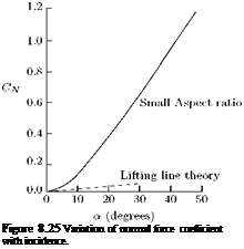
where N is the normal force. Variation of CN for JR = 1/30 with incidence angle a is shown in Figure 8.25.

For the same profile, the variation of CN, calculated with lifting line theory, with a will be as shown by the line of dashes. From Figure 8.25, it is seen that for aerofoils with very small aspect ratio the stalling incidence is very high and hence they can fly at high values of a, without stalling.

8.13.2 Zero Aspect Ratio

For the limiting case of a profile with zero aspect ratio (c ^ to) , it has been found that:

CN = 2 sin2 a.

This is the same as the behavior predicted by Isaac Newton for a flat plate which experiences a normal force proportional to the time rate of change of momentum in inelastic (incompressible) fluid particles impinging on it. In fact here we should have the normal force:

N = pV sin a • V sin a • S,

which gives the above CN.

8.13.3 The Acceleration Potential

Let us consider an aerofoil placed in a uniform flow of velocity — V in the negative direction of x-axis. We can as usual consider the aerofoil replaced by bound vortices at its surface enclosing air at rest and accompanied by a wake of free trailing vortices. Outside the region consisting of the bound vortices and the wake the flow is irrotational, and hence the flow field can be represented by a velocity potential ф such that the air velocity is given by:

q = — уф.

If the velocity induced by the vortex system is v, then:

q =—V + v.

The motion is steady, therefore the acceleration is:

If we assume[16] that the magnitude of the induced velocity v is small compared to the main flow velocity V, Equation (8.85) can be expressed, using Equation (8.83), as:

dq d

a = -(V у) q = – V-q = V— (у ф).

dx dx

Thus we have:

a = —у Ф, Ф = — V —. (8.87)

dx

where Ф is the acceleration potential. Since the velocity potential ф satisfies Laplace’s equation у2ф, it follows from Equation (8.87) that:

у2 Ф = 0. (8.88)

Assuming the flow to be incompressible and neglecting external forces, the acceleration can be expressed as:

This shows that an acceleration potential always exists. However, only with our assumption of small magnitude of induced velocity v this satisfies Laplace’s equation. Comparing Equations (8.87) and (8.89) we see that Ф and р/р can differ only by a constant, and we can take:

Ф = P—. (8.90)

P

where I is the pressure at infinity.