Our heavyweight helicopter equal in the world does not have
In Rostov started production of the most load-lifting rotary-wing car The Russian holding «Helicopt[...]

Everything about aircrafts and helicopters. News and events in aviation worldwide. Civil, transportation, military helicopters and airplanes.

Everything about aircrafts and helicopters. News and events in aviation worldwide. Civil, transportation, military helicopters and airplanes.

Everything about aircrafts and helicopters. News and events in aviation worldwide. Civil, transportation, military helicopters and airplanes.

Everything about aircrafts and helicopters. News and events in aviation worldwide. Civil, transportation, military helicopters and airplanes.


Another type of inverse problem in elastostatics is to deduce displacements and tractions on surfaces where such information is unknown or inaccessible, although the geometry of the entire 3- D configuration is given. It is often difficult and even impossible to place strain gauges and take measurements on a particular surface of a solid body cither due to its small size or geometric inaccessibility or because of the severity of the environment on that surface. With our inverse method (281) these unknown elastostatics boundary values can he deduced from additional displacement and surface traction measurements made at a finite number of points within the solid or on some other surfaces of the solid. This approach is robust and fast since it is non-iterative. A similar inverse boundary value formulation has been shown (282) to compute meaningful and accurate thermal fields during a single analysis using a straight-forw ard modification to the BEM non-linear heat conduction analysis code. An example of the concept follows using the BEM.
In general elastostatics, we can write for any discretized boundary point V and for each direction T a boundary integral equation (283|
![]() (90)
(90)
where the asterisk designates fundamental solutions and the term C| is obtained with some special treatment of the surface integral on the left hand side (283). Explicit calculation of this value can be obtained by augmenting the surface integral over the singularity that occurs when the integral includes the point V. Fortunately, explicit calculation is not necessary as it can be obtained using the ngid body motions The boundary G is discretized into Nip surface panels connected between N nodes. The functions u and p are quadratically distributed over each panel with adjacent panels sharing nodes such that there will be twice as many boundary nodes as there arc surface panels, A transformation from the global (x. y) coordinate system to a localized boundary fitted (^.r|) coordinate system is required in order to numerically integrate each surface integral using Gaussian quadrature The displacements and tractions arc defined in terms of three nodal values and three quadratic interpolation functions. The whole set of boundary integral equations can be written in matnx form (ommiting the body forces for simplicity) as
(91)
where the vector! |U| and (PI contain the nodal values of the displacement and traction vectors. Each entry in the (HJ and (G) matrices is developed by properly summing the contributions from each numerically integrated surface integral The surface tractions were allowed to he discontinuous between each neighboring surface panel to allow for proper corner treatment. The set of boundary integral equations w ill contain a total of 2N equations and 6N nodal values of displacements and surface tractions.
For a well-posed boundary value problem, at least one of the functions, u or p. will be known at each boundary node (either Dirichlct or von Neumann boundary condition) so that the equation set will be composed of 2N unknowns and 2N equations. Since there arc two distinct traction vectors at comer nodes, the boundary conditions applied there should include either two tractions or one displacement and one traction. If only displacements are specified across a corner node, special treatment is required (283).
 |
 |
|
For an ill-posed boundary value problem, both u and p should be enforced simultaneously at certain boundary nodes, while either u or p should be enforced at some of the other boundary nodes, and nothing enforced at the remaining boundary nodes. For the simple example of a quadrilateral plate with four nodes, if at two boundary nodes both u = U and p = P arc known, but at the other two nodes neither u nor p is known, the BEM equation set before any rearrangement appears as
where each of the entries in the |H) and (G) matrices is a 3×3 submatnx in 3-D elasto – statics. Straight-forward algebraic manipulation yields the following set
|
Л1І -#!2 Л14 “#I4 |
u2 |
“ЛП #11 “ЛІЗ #13 |
– /. |
|||||
|
Л22 ”#22 Л24 “#24 |
P2 |
я |
-Л2| #21 “Л23 #23 |
р 1 |
я |
/2 |
||
|
hl2 “#32 Л34 “#34 |
«4 |
“Л31 #31 “АЭЭ #33 |
р, |
/1 |
||||
|
Л42 “#42 “#44 |
Pa |
~Л41 gA[ – Л43 £43 |
Рк |
Л |
The right-hand side vector {F) is known and the left-hand side remains in the form (A)(X). Once the matrix (A) is solved, the entire u and p fields within the solid can be easily deduced from the integral formulation. The equation set |A)(X1 = (F) resulting from our inverse boundary value formulation is highly singular and most standard matrix solvers will produce an incorrect solution Singular Value Decomposition (SVD) methods [284] can be used to solve such problems accurately. The number of unknowns m the equation set need not be the same as the number of equations (284), so that virtually any combination of boundary conditions will yield at least some solution. Additional equations may be added to the equation set if u measurements are known at locations within the solid in order to enhance the accuracy of the inverse steady boundary condition algorithm. A proper physical solution will be obtained if the number of equations equals or exceeds the number of unknowns If the number of equations is less than the number of unknowns, the SVD method will find one solution, although it does not
necessarily have to he the proper solution from the physical point of view (285]. Thus, the more overspecified data is made available, the more accurate and unique the predicted boundary values will be.
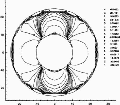
The accuracy of the inverse boundary condition code w as verified (281 ] on simple 2-D geometry consisting of an infinitely long thick-walled pipe subject to an internal gauge pressure. Тік shear modulus for this problem was G = S OxlO4 N/mm: and Poisson’s ratio was v = 0.25. The radius of the inner surface of the pipe was 10 mm and the outer radius was 25 mm The inner and outer boundaries were discretized with 12 quadratic panels each The internal gauge pressure was specified to be Pr = 100 NVmm*. while the outer boundary was specified with a zero surface traction. Figure 88 depicts a contour plot of constant values of stress tensor components Gyy that was computed using the analysis version of our second-order accurate BEM elas – tostatic code. The numerical results of this well-posed boundary value problem were then used as boundary conditions applied to the following two ill-posed problems.
|
|
Figure H8 Contours of constant stress, ayy from the wellposed analysis of an annular pressurized disk.
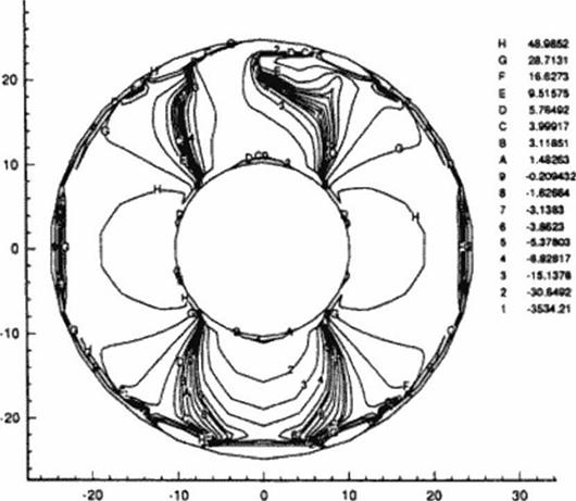
First, the displacement vectors computed on the inner circular boundary were applied as over-specified boundary conditions in addition to the surface tractions already enforced there At the same time nothing was specified on the outer circular boundary. Figure 89 represents the
contour plot of <Jvy that was obtained with our inverse boundary value ВБМ code. This stress averaged a much larger error, about 3.0%. with some asymmetry in the stress field, when compared with the analysis results.
Next, the displacement vectors computed on the outer circular boundary by the well – posed numerical analysis were used to over-specify the outer circular boundary. At the same lime nothing was specified on the inner circular boundary. Figure 90 the contour plot of ayy as computed by the inverse ВПМ technique. The predicted inner surface deformations were in error by less than 0.1%. while the predicted inner surface stresses averaged less than a 1.0% error as compared to the analysis results.
|
Figure 89 Contours of constant stress, Ojj, from the ill-posed analysis of an annular pressurized disk: inner boundary over-specified. |
It seems that an over-Specified outer boundary produces a more accurate solution than one having an over-specified inner boundary. It was also shown that as the over-specified boundary area or the resolution in the applied boundary conditions was decreased, the amount of over-specified data also decreases, and thus the accuracy of the inverse boundary v alue technique deteriorates.
H 44M52
 a «rut f!»un E «51*7»
0 S 76492
c sweir
В 111N1 А 1«Ж В -020*0?
• Ь.’бб*
7 4.1Ш
• 1W23
S 5.27«OJ « IUIV 3 -11137»
1 ЗС54Є2
1 3634.21
-L.
30
14.5 Conclusions
Siructural design of complex 3-D composite structures is possible only by using reliable optimi – zaiion codes. For simpler configurations with smaller numbers of variables it is also possible to use inverse shape design methodologies based on over-specified surface tractions and deformations. Inverse shape design and inverse boundary condition determination can be performed using both BEM and finite clement techniques. Hybrid optimization algorithms [286] that arc based on genetic evolution, simulated annealing, fu/.zy logic and neural networks and that involve manufacturing constraints (287]-(288) will be the candidates for active clastodynamic/aeroelastic control of smart structures.