Potential Equation for Bodies of Revolution

Fuselage of airplane, rocket shells, missile bodies and circular ducts are the few bodies of revolutions which are commonly used in practice. The general three-dimensional Cartesian equations can be used for these problems. But it is much simpler to use cylindrical polar coordinates than Cartesian coordi­nates. Cartesian coordinates are x, y, z and the corresponding velocity components are Vx, Vy, Vz. The cylindrical polar coordinates are x, r, в and the corresponding velocity components are Vx, Vr, Vg. For axisymmetric flows with cylindrical coordinates, the equations will be independent of в. Thus, mathe­matically, cylindrical coordinates reduce the problem to become two-dimensional. However, for flows which are not axially symmetric (e. g., missile at an angle of attack), в will be involved. The continuity equation in cylindrical coordinates is:

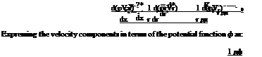
The potential Equation (9.50) can be written, in cylindrical polar coordinates, as:

Also,

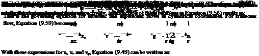
Equation (9.63) is the equation for axially symmetric transonic flows. All these equations are valid only for small perturbations, that is, for small values of angle of attack and angle of yaw (< 15°).

Conclusions

From the above discussions on potential flow theory for compressible flows, we can draw the following conclusions:

1. The small perturbation equations for subsonic and supersonic flows are linear, but for transonic flows the equation is nonlinear.

2. Subsonic and supersonic flow equations do not contain the specific heats ratio у, but transonic flow equation contains у. This shows that the results obtained for subsonic and supersonic flows, with small perturbation equations, can be applied to any gas, but this cannot be done for transonic flows.

3. All these equations are valid for slender bodies. This is true of rockets, missiles, etc.

4. These equations can also be applied to aerofoils, but not to bluff shapes like circular cylinder, etc.

5. For nonslender bodies, the flow can be calculated by using the original nonlinear equation.

9.9.1 Solution of Nonlinear Potential Equation

(i) Numerical methods.

The nonlinearity of Equation (9.49) makes it tedious to solve the equation analytically. However, solution for the equation can be obtained by numerical methods. But a numerical solution is not a general solution, and is valid only for a specific configuration of flow field with a fixed Mach number and specified geometry.

(ii) Transformation (Hodograph) methods.

When one velocity component is plotted against another velocity component, the resulting curve may be linear, whereas in the physical plane, the relation may be nonlinear. This method is used for solving certain transonic flow problems.

(iii)Similarity methods.

In these methods, the boundary conditions need to be specified for solving the equation. Detailed discussion of this method can be found in Chapter 6 on Similarity Methods.

9.5 Boundary Conditions

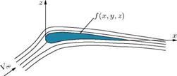
Examine the streamlines around an aerofoil kept in a flow field as shown in Figure 9.6.

In inviscid flow, the streamline near the boundary is similar to the body contour. The flow must satisfy the following boundary conditions (BCs).

Boundary condition 1 – Kinetic Bow condition

The flow velocity at all surface points are tangential on the body contour. The component of velocity normal to the body contour is zero.

Boundary condition 2

At z ^ ±x, perturbation velocities are zero or finite. The kinematic flow condition for the aerofoil shown in Figure 9.6, with small perturbation assumptions, may be written as follows.

Body contour: f = f (x, y, z)

The velocity vector V at any point on the body is tangential to the surface. Therefore, on the surface of the aerofoil, (V • vf) = 0, that is:

where the subscript “c” refers to the body contour and (dz/dx) is the slope of the body, and u and v are the tangential and normal components of velocity, respectively. Expressing u and w as power series of z, we get:

u(x, z) = u(x, 0) + az + a2z2 + … w(x, z) = w(x, 0) + hiz + b2z2 + …

The coefficients a’s and h’s in these series are functions of x. If the body is sufficiently slender:

w(x, 0) _ ( dz^

Vx + u(x, 0) (dx ) C

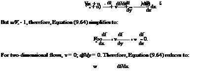
that is, for sufficiently slender bodies, it is not necessary to fulfill the boundary condition on the contour of the aerofoil. It is sufficient if the boundary condition on the x—axis of the body is satisfied, that is, on the axis of a body of revolution or the chord of an aerofoil. With u/Vx ^ 1, the above condition becomes:

that is, the condition is satisfied in the plane of the body. In Equations (9.67) and (9.68), the elevation of the body above the x—axis is neglected.

9.10.1 Bodies of Revolution

For bodies of revolution, the term 1 d (rvr) present in the continuity equation (9.54) becomes finite. Because of this term, the perturbations near the body become significant. Therefore, a power series for velocity components is not possible. However, we can apply the following approximation to express the perturbation velocity as a power series. For axisymmetric bodies:

From the above discussions, it may be summarized that the boundary conditions for this kind of problem are the following.

For two-dimensional (planar) bodies:

(Vw ) *	y (w)o _		(9-71)
V + u ‘ c	V»	Kdx ) c
For bodies of revolution (elongated bodies):
R(x) Vr 1 ^	^ (rVr)o _	R() dR(x) = R(x) , •	(9-72)
v V» + u ‘ c	V»	dx