Computational Algorithm and Boundary Conditions

For time marching computation in the elliptic coordinates region of the computa­tional domain, Eqs. (15.42) to (15.45) are first rewritten in the д – в coordinates as in Section 5.6. The derivatives are then discretized according to the 7-point stencil DRP scheme. At the mesh-size change boundaries, the multi-size-mesh multi-time-step

DRP scheme of Chapter 12 is implemented. This scheme allows a smooth connec­tion and transfer of the computed results using two different size meshes on the two sides of the boundary. It also allows a change in the size of the time step (see Figure 15.25). This makes it possible to maintain numerical stability without being forced to use very small time steps in subdomains where the mesh size is large. This results in a very efficient computation without loss of accuracy as noted in Chapter 12.

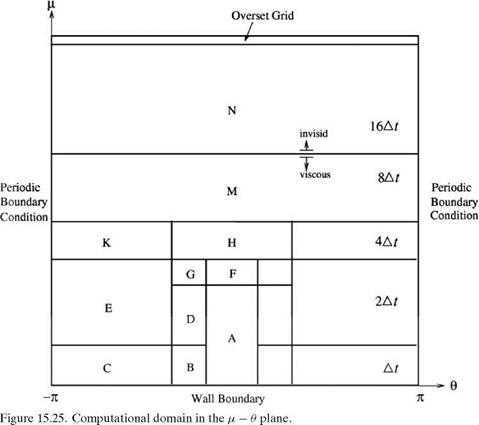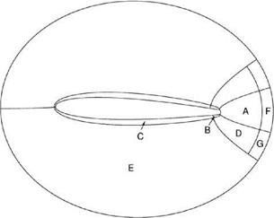
Figure 15.26. Various subdomains in the physical space.

On the left, the top and bottom boundaries of the computation domain shown in Figure 15.24, the radiation boundary conditions of Section 6.5 are imposed. On the right boundary, outflow boundary conditions of Section 6.5 are enforced. On the airfoil surface, the no-slip boundary conditions are used. This, however, will create an overdetermined system of equations if all the discretized governing equations are required to be satisfied at the boundary points. To avoid this problem, the two momentum equations of the Navier-Stokes equations are not enforced at the wall boundary points. The continuity and energy equations are, nevertheless, computed to provide values of density, p, and pressure, p, at the airfoil surface. This way of enforcing the no-slip boundary conditions was discussed at the end of Section 6.7.