Computation of Axisymmetric Jet Screech

For the purpose of illustrating the essential steps and considerations needed to simulate jet screech computationally, only axisymmetric jet screech is considered (see Shen and Tam, 1998). This is to keep the discussion to a reasonable length. For axisymmetric jet screech associated with jets issued from a convergent nozzle, the jet Mach number is restricted to the range of 1.0 to 1.25. Numerical simulation of jet noise generation is not a straightforward undertaking. Tam (1995) had discussed some of the major computational difficulties anticipated in such an effort. First of all, the problem is characterized by very disparate length scales. For instance, the acoustic wavelength of the screech tone is more than 20 times larger than the initial thickness of the jet mixing layer that supports the instability waves. Furthermore, there is also a large disparity between the magnitude of the fluid particle velocity of the radiated sound and the velocity of the jet flow. Typically, they are five to six orders of magnitude different. To be able to compute accurately the instability waves and the radiated sound, a highly accurate CAA algorithm with shock-capturing capability as well as a set of high-quality numerical boundary conditions are required.

15.6.1.1 Computational Model

For an accurate simulation of jet screech generation, it is essential that the feedback loop be modeled and computed correctly. The important elements that form the feedback loop are the shock cell structure, the large-scale instability wave, and the feedback acoustic waves. In the mixing layer of the jet, turbulence is responsible for its spreading. The spreading rate of the jet affects the spatial growth and decay of the instability wave. Thus, turbulence in the jet plays an indirect but still important role in the feedback loop. The length scales of the instability wave, the shock cells,

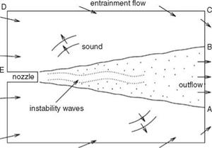
Figure 15.53. A sketch of the physical domain to be simulated.

as well as the feedback acoustic waves are much longer than that of the fine-scale turbulence in the mixing layer of the jet. Because of this disparity in length scales, no attempt is made here to resolve the fine-scale turbulence computationally. Based on these considerations, an unsteady RANS model is regarded as adequate. To provide the necessary jet spreading induced by turbulence, the к – e turbulence model is adopted. Here, the к — є model simulates the effect of the fine-scale turbulence on the jet mean flow. In the computation described below, the modified к – e model of Thies and Tam (1996), optimized for jet flows, is used.

Figure 15.53 shows the physical domain to be simulated. The following scales are used in the computations; length scale = D (nozzle exit diameter), velocity scale = aTO (ambient sound speed), time scale = D/aTO, density scale = pTO (ambient gas density), pressure scale pTOa^, temperature scale = TTO (ambient gas temperature); scales for к, e, and ut are a^, a3/D, and aTOD, respectively. The dimensionless governing equations in Cartesian tensor notation in conservation form are as follows:

In these equations, y is the ratio of specific heats, и is the molecular kinematic viscosity. k0 = 10—6 and e0 = 10—4 are small positive numbers to prevent division by zero. The model constants are given in Section 15.5.2. The inverse molecular Reynolds number v/(amD) is assigned a value of 1.7 x 10—6 in the computation. Note that, for the range of Mach numbers and jet temperatures considered, the Pope and Sarkar corrections often added to the k – e model are not necessary and are omitted. Here, only cold jets are considered. For this reason, the Tam and Ganesan hot-jet correction is not needed. Outside the jet flow both k and e are zero. On neglecting the molecular viscosity terms, the governing equations become the Euler equations.