ALLOWANCE FOR PARASITE DRAG

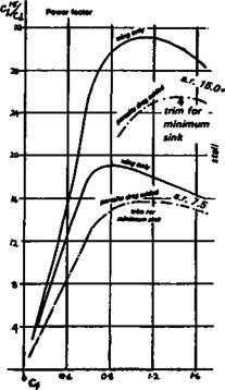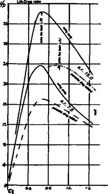
After correcting wind tunnel results for aspect ratio effects, to arrive at an estimate of drag for the whole model, parasite drag must be taken into account This may be estimated from tunnel tests on fuselages, undercarriages, etc. with an additional quantity for interference drag. As a rule such detailed estimates are not necessary for modelling. To illustrate the effect of parasite drag on performance, however, the above example is taken further. It is assumed (arbitrarily but not unreasonably) that the model with a. r. 7.5 of the previous example has a parasite drag coefficient of 0.01, this remaining constant throughout the flight attitudes considered. This assumption breaks down if the fuselage is not aligned with the average flow direction, but is sufficiently accurate for purposes of illustration.

Fig. A4 Aspect ratio and parasite drag effects

Note: parasite drag has a considerable effect on the trim for best performance, shifting the peaks of the curves to the higher Cl (higher angle of attack) side.

The calculation proceeds as before: the parasitic increment of drag is added to the total of profile and induced drag, to give the total drag coefficient of the whole model. This new total is then used to work out the model power factor and L/D.

1	2	3	4	5	6
Cl	Cdi x Cap	Add parasite V’ci3	у/ ci3/Cd	Ci/Cl
	a. r. 7.5	Cd = .01		Total
.4	.01879	.02879	0.253	8.788	13.89
.6	.02508	.03508	0.465	13.255	ІГШ	Max. L/D
.8	.03726	.04726	0.716	15.150	16.93
1.0	.05314	.06314	1.000	15.837	15.84
1.2	.07245	.08245	1.315	115.9491	14.55	Max. Power Factor
1.4	.09568	.10568	1.657	15.679	13.25
1.5	.10919	.11919	1.837	15.412	12.58
1.6	.12354	13354	2.024	15.156	11.98
1.675	.13545	.14545	2.168	14.905	11.52

The power factor and L/D worked out in columns 5 and 6 are graphed and from this graph the desired Cl for trimming is found. The values for a. r. 15 are also plotted for comparison (Fig. A4).

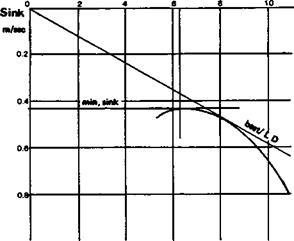
Assuming the model weight and wing area are known, the sinking speed can be computed and plotted as shown to give the ‘polar1 curve of the model. This gives the minimum sinking speed by inspection. The sinking speed of a model glider (from page

232) is given by j-^—————- £-

Sinking speed =y—

Assuming a model wing loading of W/S = 3 kg/sq. m, the first term becomes 6.932. Thus sinking speed at each Cl and V value is as shown for the a. r. 7.5 model: 1 2 3 4 Cl Vm/sec 1/CL15/Cd Sinking Speed, M/Sec .4 10.96 0.11379 .7895 .6 8.9 0.07544 .5229 .8 7.75 0.06601 .4576 1.0 6.93 0.06314 .4377 1.2 6.33 0.06269 .4346* ‘MINIMUM SINK 1.4 5.86 0.06378 .4421 1.5 5.66 0.06488 .4498 1.6 5.48 0.06598 .4574 1.675 5.36 0.06709 .4651

A more complete performance estimate may be attempted if full wind tunnel test results are available for the aerofoil to be used. Interesting studies are possible to illustrate the effect of increased wing loading and aspect ratio. If the wing loading is increased, the glider flies faster, which raises the Re and may improve the drag characteristics of the aerofoil. Given complete tunnel results this improvement may be estimated, and the profile drag figures in the calculation table will show the difference. Whether the improvement in profile drag is enough to offset the increased sinking speed due to the higher wing loading will depend entirely on the aerofoil and how much it is affected by the ‘ increased Re. Similarly, with a model of given wing area and wing loading, increasing the aspect ratio decreases induced drag but reduces Re, and so increases profile drag. Given adequate wind tunnel tests results, it is possible to compute the effects on model performance of such changes, and so determine the best aspect ratio.

Some examples have been published by the author and are listed among the references at the end of Chapter 10.

As an illustration of the results possible, the following tables and polar curve are included, but a full explanation of die method would occupy too much space.

Velocity, M/sec: 8.30 Mean Reynolds number 113043 Root angle of attack 15.721 Cl Chord Re number Profile Cd 1.09 0.210 119345 0.02062 1.09 0.210 119345 0.02062 1.08 0.210 119345 0.02055 1.05 0.210 119345 0.01950 1.02 0.203 115634 0.03117 1.00 0.192 109108 0.03355 0.94 0.182 103534 0.03430 0.84 0.174 99050 0.03280 0.65 0.169 95766 0.03212 0.37 0.165 93763 0.02542

THE DRAG BUDGET

Figure 4.9 was produced by applying the methods outlined above. The contribution of each type of drag to the model Cd at each Cl may easily be found in the foregoing tables;

245

□ WING A = 20 ★ WING3A=8
POLARS	■ WING 2 A* 14
M/S “ 4.3kQ/m*

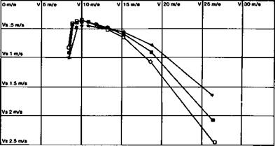
Fig. A6 Polar curves of three sailplane wings of different aspect ratios but all of the same aerofoil section.

[The low A models are ballasted to bring them to the same M/S as the A = 20 model.] Note the marked superiority of the [ballasted] A = 8 model at high speed. At low speed there is little to choose between A = 14 [ballasted] and A = 20. The low Re of the high A wing is responsible.

these are entered in the table below.

To find the dragforce contributed at each flying speed, first the velocity of flight at each Cl is found by applying the standard formula:

= / W x 9.81 / 3 x 9.81 = /48.048

л/liSx 1.225 Cl w й x 1.225 x 1 x Cl * Cl

For the purpose of the example calculation, W/S (wing loading) was assumed 3 kg./sq. metre (approx. 9.8 ozs./sq. ft), and a model weight of 3kg. assumed (6.6151bs.).

Next, each Cd is multiplied by VipSV2 to produce drag force in kg. The results are of course only approximate since no proper allowance has been made for varying Re. The assumed model would achieve Re approx. 280,000 to match the wind tunnel results if its VL (velocity multiplied by chord) was about 4. This corresponds to a model with chord 0.3 metres flying at 13.3 metres per second (11.8 ins. at 29.8 m. p.h.). As the figures below show, the model would reach this speed at Cl between 0.2 and 0.4. The aspect ratio of 7.5 gives a span of 2.74 metres, wing area 1 sq. metre.

The drag budget is worked out in the table overleaf, and plotted as in Figure 4.9.