Stalling

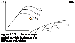
We know that the lift coefficient CL is a function of the absolute angle of incidence a, and strongly influenced by the Reynolds number Re = pVl/д. For a given aircraft we could therefore draw a surface which is the locus of the point (CL, a, Re) which is the characteristic lift surface for that aircraft. Since the aircraft is given, l is known, and for the freestream flow the state of the air is given, so that in this case CL is a function of incidence a and of the forward speed V. From this point of view the characteristic surface may then be regarded as the locus of the point (CL, a, V). Let us consider three points on this surface (CL1, aj, Vj), (CL2, a2, V2), (CL3, a3, V3), where let us suppose V1 < V2 < V3 and a < a2 < a3. The variation of CL with a corresponding to velocities V, V2, V3 are shown in Figure 10.3.

It is seen that the straight portions of CL versus a graph corresponding to values of V, V2, V3 of V, the straight portions are practically in the same line. This plot may be thought of as showing sections of the characteristic surface by planes V = V, V = V2, V = V3. In all our discussions in the previous chapters, we considered CL to be directly proportional to a, that is, we have restricted ourselves to the linear part of the graph about which pure theory can make statements. Plots of the type shown in Figure 10.3 must necessarily be obtained from experimental measurements, and the graph shows that, with increasing incidence, CL rises to a maximum value CLmax and then decreases.

It is generally, but not always, the case that CLmax for a given V increases as V increases. If the sections of the characteristic surface by the planes a = a1, a = a2, a = a3, we get the variation of CL with V as shown in Figure 10.4.

у

Figure 10.4 Lift curve slope variation with V in the sections of the characteristic surface cut by the planes a = аь

a = a2, a = a3.

The stalled state is that in which the airflow on the suction side of the aerofoil is turbulent. It is found that, just before the stalled state sets in, the lift coefficient attains its maximum value, and the corresponding speed is called the stalling speed. Thus the stalling speed corresponding to a given CLmax can be read from the continuous curve of Figure 10.4.

Stalling speed is a function of incidence. Variation of a with V in the sections of the characteristic surface by planes CL = CL1, CL = CL2, CL = CL3 is as shown in Figure 10.5.

In Figure 10.5 the continuous line shows the stalling speed as a function of the stalling incidence aS. Any point (a, V) above this curve corresponds to stalling flight, any point below it with normal flight.

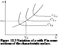It should be noted that the foregoing discussion only applies to speeds V such that the flow speed over the aerofoil nowhere approaches the speed of sound, that is, we neglect variation with Mach number.

The graphs of the above type are all cases deduced from experiments, generally in wind tunnels for condition corresponding to linear flight at constant speed. When the aircraft flies in a curved path the graph will differ slightly from the above, but investigations made by Wieselsberger [Reference 9] show that the changes are of the order of the square of the ratio of the span to radius of curvature of the path and may therefore, in general, be neglected.

Moreover, for most calculations it is sufficient to substitute one of the CL graphs in Figure 10.3 for the whole graph, namely the one which corresponds to the landing speed, because the danger of stalling is generally greatest when the aircraft is about to land and is therefore flying near to the stalling incidence and at a low speed. When we substitute Reynolds number Re for velocity throughout, the foregoing conditions may be held to apply to a family of geometrically similar aircraft. For such a family there will be one characteristic lift surface.