Our heavyweight helicopter equal in the world does not have
In Rostov started production of the most load-lifting rotary-wing car The Russian holding «Helicopt[...]

Everything about aircrafts and helicopters. News and events in aviation worldwide. Civil, transportation, military helicopters and airplanes.

Everything about aircrafts and helicopters. News and events in aviation worldwide. Civil, transportation, military helicopters and airplanes.

Everything about aircrafts and helicopters. News and events in aviation worldwide. Civil, transportation, military helicopters and airplanes.

Everything about aircrafts and helicopters. News and events in aviation worldwide. Civil, transportation, military helicopters and airplanes.


In many aeroacoustics problems, it is sometimes advantageous to compute the mean flow first and then to turn the noise sources on and compute the sound field using the same computer code. This becomes a necessity if the sound intensity is very low; smaller than the error of the numerical mean flow solution (in comparison with the exact solution). One drawback of this approach is that it could take a long time to converge to a steady state when using an almost nondissipative computation scheme such as the dispersion-relation-preserving (DRP) scheme. On the other hand, using a more dissipative scheme might damp out the sound. Because of the nearly nondissipative nature of the scheme, the only way by which the residual associated with the initial condition can be reduced to a very low level is to have it expelled slowly through the boundaries of the computational domain. This sometimes could take a very long computation time. A method to achieve accelerated convergence to steady state without compromising accuracy would, therefore, be very useful.
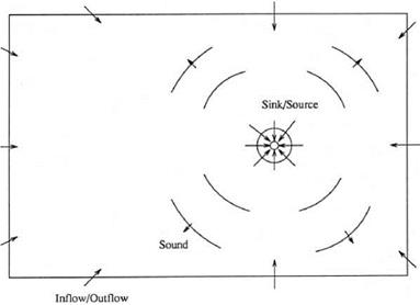
To illustrate a way to attain accelerated convergence to steady state, consider a two-part problem of computing the mean flow created by a localized sink/source and then the sound field created by tiny oscillations of the sink/source strength. The problem is as shown in Figure E1. In two dimensions, the governing equations are as follows:
|
Figure E1. Acoustic radiation from an oscillatory sink/source flow. |
In Eq. (E5) (x0, y0) are the coordinates of the center of the sink/source. Nondimensional variables with a0 (sound speed) as the velocity scale, Ax as the length scale, Ax/a0 as the time scale, p0 as the density scale, and p0a0 as the pressure scale are used in all computations.
In this illustration, the computational domain of Figure E1 is discretized by using a square mesh with Ax = Ay. A120 x 100 computational grid centered at the origin of coordinates is used. The following values are assigned to the source parameters:
a = І36:, r0 = 12, Q = 0.0456, x0 = 20, y0 = 0.
To start the mean flow computation, a zero initial condition is used. The solution is time marched to a steady state by means of the 7-point stencil DRP scheme. Artificial selective damping with a mesh Reynolds number (RAx = a°7^) equal to
a
10 is added to the discretized equations. With such a small amount of damping, in a trial computation, the residual is able to settle down over time to a magnitude of the order of 10-13 (the residual is effectively the value of the time derivative or its finite difference approximation). This is just the machine truncation accuracy (single precision). This very low background noise level is, however, a necessary condition for performing the subsequent computation of the very low intensity sound (of the order of 10-10) produced by extremely tiny oscillations of the sink/source strength.
Through numerical experimentation, the following technique referred to as the “canceling the residuals” has been found to be very effective in promoting accelerated convergence. Since the difference between the numerical and the exact solution is of the order of a percent, further time marching calculation is a waste of effort in terms of improving the accuracy of the numerical solution, once the residuals reach a level of order 10-5. With this in mind, it is possible to add terms that are exactly equal in magnitude, but opposite in sign to the residuals to the right side of
|
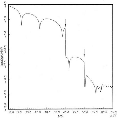
Figure E2. Time history of the residual of the м-velocity component at the grid point (-20, -25). Arrows indicate the application of the canceling-the-residuals technique for accelerated convergence. |
each of the governing equation. These are terms of order 10-5 or less and would, therefore, not materially affect the accuracy of the steady-state numerical solution. The added terms may be regarded as minute artificial distributed sources of fluid, momentum, or heat. The consequence of adding these minute source terms is to render the residuals instantaneously to zero. Of course, for a multilevel marching scheme, the residuals of the scheme are greatly reduced in this way, but they would not be exactly equal to zero at the next time level. Numerical experiments indicate that when this canceling-the-residuals procedure is performed, the overall residual of the computation drops almost instantaneously by several orders of magnitude. This method can be applied repeatedly until machine accuracy is achieved.
Figure E2 shows the time history of the residual, log10 | d |, at the point (-20,-25). The arrows in this figure indicate when the canceling-the-residuals technique is applied. It is clear that there is a dramatic decrease (of 3 to 4 orders of magnitude) in the residual immediately after each application of the method.
|
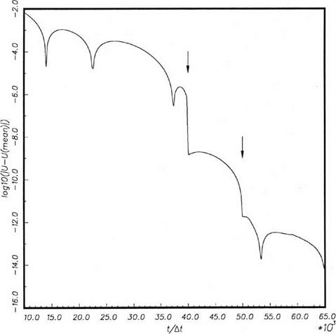
Figure E3. Convergence history of the м-velocity component at the point (+20, -25). Arrows indicate the application of the canceling-the-residuals technique for accelerated convergence. |
Figure E3 shows the corresponding convergence history of the м-velocity component at the mesh point (+20, -25). The computed solution rapidly approaches the eventual mean value of the velocity component right after each application of the accelerated convergence technique. It is worthwhile to mention that the method works in all the cases that have been tested. The total computer run time needed to attain a steady-state numerical solution is drastically reduced in each instance.