CONTROL SYSTEM: STABILITY, ROUTH-HURWITZ

CRITERION, NYQUIST CRITERION, GAIN/PHASE MARGINS

A linear spring-mass system is described as (Figure 2.5)

Mx + Dx + Kx = 0 (C1)

Assume that mass M is displaced to the right by a small disturbance x. When the displacement takes place, the spring with its stiffness K (if K is positive) will provide a restoring force proportional to Kx to the mass. The positive restoring force is because K is positive and it is in the direction opposite to the initial movement of the object. The mass will have an initial tendency to move toward the original position. This is the static stability of a dynamic system. If K is negative then naturally the mass will keep moving in the forward direction, since the spring force will be in the direction of x. The mass will further move away from the original equilibrium

TABLE C1

Steady-State Error for Types of Systems

	Type "0"	Type "1"	Type"
Step input u(t) = 1	1/(1 + K)	0	0
Ramp input u(t) = t	1	1/K	0
Acceleration input u(t) = 212	1	1	1/K

rr

position. This condition is called static instability. The differential Equation C1 has two roots:

Routh-Hurwitz Criterion

The characteristic equation of the control system is its denominator equated to zero. The Routh-Hurwitz (RH) criterion relates to studying the characteristic equation: (1) the control system is dynamically stable if all the roots have negative real parts, (2) the system is unstable if any root has a positive real part, and (3) the system is neutrally or marginally (stable/unstable) if one or more roots have pure imaginary values. Let this equation be given as g(s) = ansn + an-1sn-1 + ••• + a1s + a0. Now, construct the Routh array as shown. The first two rows are obtained from the characteristic equation. The remaining element of the Routh array are calculated from the following expressions: bn-1

1-. an-1an-4 anan-5 • ~ .

bn-3 =———————— ~1—————– ; —Cn—1~———— b„-1

the sign changes in the elements of the first column of the array. This number signifies the number of roots with positive real parts. If there are no sign changes, then the system is stable.

sn sn-1 sn-2 sn-3	an	an – 2	an—4 – – –
an – 1 bn – 1	an – 3 bn – 3	an-5 – – – bn—5 – – –
Cn— 1	Cn—3	Cn—5 – – –
s0	hn— 1

Nyquist Criterion

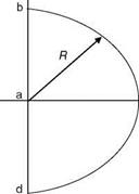
We can examine the frequency response of the G(s)H(s) (or GH(s)) loop TF and see if the gain is greater than unity at the phase lag of 180°. This is equivalent to studying the condition GH( jv) = -1 or finding a root of (GH + 1) on the s-plane jv axis, this being the stability boundary. The stability of the system is studied by using the principle of an argument advanced by Nyquist. A semicircular contour of infinite radius is used to enclose the right hand s-plane (RHS). According to this principle, as s traverses the closed contour in a clockwise direction, the increment in the argument

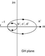FIGURE C1 Nyquist contour (R is infinite radius) and Nyquist plot.

of (1 + GH) is 2pN. Now, if P = the number of the poles of GH + 1 and Z = the number of zeros of GH + 1 inside the Nyquist contour (i. e., the right hand s-plane with infinite radius), then N = P — Z, the number of counterclockwise encirclements of the origin of the s-plane. This can be translated to count the encirclements of the critical point — 1 + j0 by the GH. The stability criterion is specified as Z = P — N. We recognize here that the poles of 1 + GH are the open loop poles and the zeros of 1 + GH are the closed loop poles. Thus, the number of the unstable closed loop poles is equal to the number of the unstable open loop minus the number of the counter­clockwise encirclements of the critical point. The steps involved in the determination of the stability of the system using the Nyquist plot are illustrated in Figure C1 for the following TF [1]:

(s + 1)(s + 2)(s + 5)’

(1) The part ab of the Nyquist contour is the jv axis from v = 0 to v = 1. This maps to the Nyquist polar from a’ to b’ (the latter at the origin), (2) The infinite semicircle bcd maps into the origin of the polar plot of GH = plane, i. e., into points b’, c’, and d’, and (3) The negative jv axis da maps into the curve d’a’ in the GH-plane. We see that the GH-plane Nyquist plot does not enclose the critical point, and hence N = 0. Since P = 0 (there are no poles of the GH in the RHS plane) hence Z = 0, meaning that there are no closed loop poles in the RHS plane. The closed loop system is stable.

Gain/Phase Margins

We see from the RH criterion that it gives the absolute stability of the system, i. e., whether the system is stable or unstable. The gain/phase margins give the relative stability of the system. They measure the nearness of the open loop frequency response to the critical point. The gain margin (the GH frequency response is plotted)
from the point where the phase lag is 180°, is the additional gain needed to make the system just unstable, whereas the phase margin (from the point where the gain is one) is the additional phase lag needed to render the system just unstable. The margins for a given system can be easily computed using the MATLAB control system toolbox. Gain and phase margins are the criteria specified for the design of control systems. What is almost always specified is that the gain margin (of the loop TF GH(s)) should be at least 6 dB, and the phase margin should be at least 45°.