Reduced Order Modelling

5.2 Introduction

It was shown in section §4 how the analysis tools presented in section §5 can provide a useful means by which the analysis methodology outlined in section §3 can help guide kinematic modelling. However, the final goal, as evoked in the introduction, is to understand and model the dynamic law associated with sound production, as it is only then that one can really claim to have identified source mechanisms.

In this section we provide a very brief introduction to reduced order modelling. For a more complete treatment the reader is encouraged to refer to Noack et al. (2011).

5.3 Two approaches for reduced order dynamical modelling

The governing dynamic law of the full flow system is:

N q = 0. (180)

The objective of reduced order modelling, the final stage of the analysis methodology outlined in section §3, is to construct a simplified dynamic law governing the evolution of a simplified kinematic field, q:

Nq = o. (181)

Two reduced-order dynamic modelling strategies will be outlined here. The first is useful when relatively complete space-time data is available, from a numerical simulation for example, the second being useful in an experimental context, where more limited data is available. In both cases the objective is to write down an Ordinary Differential Equation that mimics either the dynamics of the Navier Stokes operator, or of some reduced sub­space of the system.

This can be achieved once the flow has been expanded in terms of a set of orthogonal basis functions, which can be obtained, for example, by means of POD:[21]

N

q(x, t) = ^2 Oi(t)0(x). (182)

n=1

The temporal evolution of the flow is here contained in a. j(t), and so it is via these, the topos, that we can attempt to write down a simplified

evolution equation, in the form of an ODE:

which mimics both linear and non-linear aspects of the dynamics, via, re­spectively, the first and second terms on the right hand side. The goal is to compute the coefficients, Lij and Qijk, that best reproduce the (known) temporal structure of ai (t); we then have a simplified dynamic model for the flow (or flow sub-space) considered.

The difference between the two said approaches is in the way that the coefficients Lij and Qijk are computed.

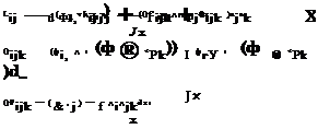
Galerkin projection In this approach, the Navier Stokes equations are projected onto the basis functions, ф(х), giving, directly

Qijk is here associated with the non-linear convection term of the Navier – Stokes equations, QPjk is associated with the pressure term[22], while Lij is associated with viscous and linear convection terms.

Polynomial identification This technique, proposed by Perret et al. (2006) is useful when only limited experimental data is available. The poly­nomial form

Lij aj + Qijk aj ak

is chosen as a suitable generic dynamic ansatz; then, knowing the values of ai, we have a linear system of equations with unknowns, Lij and Qijk. By solving this linear system, the coefficients can be identified.

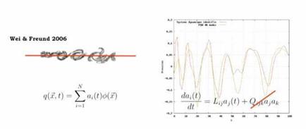
Figure 33. Left: instantaneous image of DNS of 2-D mixing-layer of Wei and Freund (2006): pressure fluctuations are sampled along the red line, and this field is then decomposed using POD; Right: green line shows a truncated representation of the DNS solution for the spatial structure of the pressure field on the red line at some given instant in time, while the red line shows the structure predicted by the simplified dynamic model given by the ODE—the quadratic term has been neglected in this example.