THE MEANING OF PROBABILITY AND DISTRIBUTION FUNCTION

Consider a very simple experiment of tossing a coin and observing whether a “head” turns up. If we make n throws in which the “head” turns up v times, the ratio vjn may be called the frequency ratio or simply the frequency of the event “head” in the sequence formed by the n throws. It is a general experience that the frequency ratio shows a marked tendency to become more or less constant for large values of n. In the coin experiment, the frequency ratio of “head” approaches a value very close

to Vs-

This stability of the frequency ratios seems to be an old experience for long series of repeated experiments performed under uniform conditions. It is thus reasonable to assume that, to any event £ connected with a random experiment S, we should be able to ascribe a number P such that, in a long series of repetitions of S, the frequency of occurrence of the event E would be approximately equal to P. This number P is the probability of the event E with respect to the random experiment S. Since the frequency ratio must satisfy the relation 0 < vjn < 1, P must satisfy the inequality

0 < P < 1 (1)

If an event E is an impossible event, i. e., it can never occur in the performance of an experiment S, then its probability P is zero. On the other hand, if P = 0 for some event E, E is not necessarily an impossible event. But, if the experiment is performed one single time, it can be considered as practically certain that E will not occur.

Similarly, if £ is a certain event, then P = 1. If P = 1, we cannot infer that £ is certain, but we can say that, in the long run, £ will occur in all but a very small percentage of cases.

The statistical nature of a random variable is characterized by its distribution function. To explain the meaning of the distribution function, let us consider a set of gust records similar to the one presented in Fig. 8.6. Let each record represent a definite interval of time. Suppose that we are interested in the maximum value of the gust speed in each record. This maximum value will be called “gust speed” for conciseness and will be denoted by y. The gust speed varies from one record to another. For a set of data consisting of n records, let v be the number in which the gust speed is less than or equal to a fixed number x. Then vjn is the frequency ratio for the statement у < x. If the total number of records n is increased without limit, then, according to the frequency interpretation of probability, the ratio v/n tends to a stationary value which represents the probability of the event “y < x.” This probability, as a function of x, will be denoted by

P(y^x) = F(x) (2)

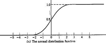
The process can be repeated for other values of x until the whole range of x from — oo to oo is covered. The function F(x) defined in this manner is called the distribution function of the random variable y.

Obviously F(x) is a nondecreasing function, and

F(- oo) = 0, 0 < F(x) < 1, F(+ oo) == 1 (3)

If the derivative F'(x) — f(x) exists, fix) is called the probability density or the frequency function of the distribution. Any frequency function f{x) is nonnegative and has the integral 1 over (— oo, oo). Since the difference Fib) — F(a) represents the probability that the variable у assumes a value belonging to the interval a <y < h,

P(a < у < b) = F(b) – F(a) (4)

In the limit it is seen that the probability that the variable у assumes a value belonging to the interval

x < у < x + Ax

is, for small Ax, asymptotically equal to f(x) Ax, which is written in the usual differential notation:

P(x < у < x + dx) — f(x) dx

In the following, we shall assume that the frequency function fix) = F’ix) exists and is continuous for all values of x. The distribution function is then

if absolutely convergent, are called the first, second, third, • • ■ moment of the distribution function according as v = 1, 2, 3 • • • respectively. The first moment, called the mean, is often denoted by the letter m

m = f хДх) dx (8)

J — oo

The integrals

Л 00

Uv = I (x — mf f(pc) dx (9)

J — CO

are called the central moments. Developing the factor (x — my according to the binomial theorem, we find

fi0 = 1

^i = 0

/4 2 = <*2 — (50)

ys = «з — 3ma2 + 2 rtf

Measures of location and Dispersion. The mean m is a kind of measure of the “location” of the variable y. If the frequency function is inter­preted as the mass per unit length of a straight wire extending from — oo to – f oo, then the mean m is the abscissa of the center of gravity of the mass distribution.

The second central moment gives an idea of how widely the values of the variable are spread on either side of the mean. This is called the variance of the variable, and represents the centroidal moment of inertia of the mass distribution referred to above. We shall always have > 0. In the mass-distribution analogy, the moment of inertia vanishes only if the whole mass is concentrated in the single point x = m. Generally, the smaller the variance, the greater the concentration, and vice versa.

In order to obtain a characteristic quantity which is of the same dimen­sion as the random variable, the standard deviation, denoted by a, is defined, as the nonnegative square root of

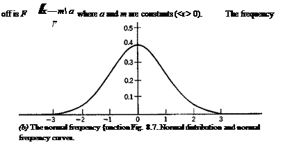
The corresponding normal frequency function is

f(x) = – l=e-*al* (13)

V 27Г

Diagrams of these functions are given in Fig. 8.7. The mean value of the distribution is 0, and the standard deviation is 1.

A random variable f will be said to be normally distributed with the parameters m and a, or briefly normal (m, a) if the distribution function

F(x)

f(x)

function is then

(14)

It is easy to verify that m is the mean, and a is the standard deviation of the variable f.

Note that, in the normal distribution, the distribution function is completely characterized by the mean and the standard deviation.