Our heavyweight helicopter equal in the world does not have
In Rostov started production of the most load-lifting rotary-wing car The Russian holding «Helicopt[...]

Everything about aircrafts and helicopters. News and events in aviation worldwide. Civil, transportation, military helicopters and airplanes.

Everything about aircrafts and helicopters. News and events in aviation worldwide. Civil, transportation, military helicopters and airplanes.

Everything about aircrafts and helicopters. News and events in aviation worldwide. Civil, transportation, military helicopters and airplanes.

Everything about aircrafts and helicopters. News and events in aviation worldwide. Civil, transportation, military helicopters and airplanes.


An FCS can have various roles to play: (1) automatic pilot controller—autopilot,
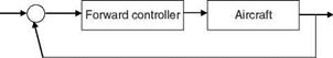
(2) basic stability augmentation, (3) guidance control loop, and (4) FBW/FCS for high-performance fighter or even transport aircraft (like AIRBUS 320). In any case, control deflection would be applied, which is proportional to the deviation of the aircraft, say, in the attitude from the reference value (Figure 8.1). New situations and developments paved the way for intense research in flight mechanics and control [3]: (1) increased wing loading, (2) mass concentration in the slender fuselages,
(3) swept/delta wing aircraft, (4) hydraulic powered controls, and (5) introduction of turbojet engines. These basic changes in the design of aircraft were required to expand the flight envelope of the aircraft and to enhance the performance of the aircraft [3]. This resulted in deficiency in stability and control characteristics of the aircraft, which further gave impetus to the design and development of sophisticated FBW/FCS. In order to handle the large hinge moments of the control surfaces, hydraulic and related control systems came into use, which increasingly ‘‘distanced’’ the pilot from the ‘‘feel’’ of the aerodynamic forces acting on the control surfaces. This further introduced the use of the artificial feel system to aid the pilot in performing the control task. A modern high-performance fighter aircraft would have full authority FBS/FCS, which would cater not only to the basic stabilization task but also to many tasks that allow for care-free maneuvering of the aircraft and provide overall best aerodynamic efficiency. Any FCS would be based on some control strategies that are described next [3-5].
With three-axis attitude stabilization, a feasible mechanization of flight control would be attitude rate and attitude stabilization—attitude hold—when no command is given. This leads to ‘‘rate command/attitude hold’’ system and the pilot’s task of stabilization of the aircraft is either eliminated or drastically reduced. A control system strategy based on U or a and 8e stabilizes the angular motion of an aircraft. In (U, 8e) strategy, the U is kept constant and the inherently unstable aircraft is made stable. The attitude response of the aircraft due to gust inputs can be reduced.
|
вс ве Se
FIGURE 8.1 Attitude stabilization control system. |
This helps reduce the pilot’s workload. In the case of the control strategy based on (a, 8e), the airflow direction relative to the aircraft is maintained constant. However, the pilot cannot get the feel of the AOA, since it cannot be visualized from the out-ofwindow view. Another demerit is that AOA measurements could often be inaccurate. The alternative control strategy based on (nz, 8e) would maintain the load factor constant. Over and above the foregoing control strategies, a system based on u and engine thrust can be used to ‘‘stabilize’’ the airspeed. This strategy, however, has a demerit during takeoff and initial climb phases because maximum thrust is demanded. Yet another control strategy is to use a direct-lift (aerodynamic) control surface to effect changes in the flight path angle. The (g, 8e) TF is given by
With a small value of na, there would be a large lag in the variation of g after the change in pitch attitude has occurred. Also, the small value of na requires large AOA changes and hence large pitch angle changes. In the above situation limited use of the direct-lift control strategy would be useful due to increase in drag, thereby restricting the use in the approach and landing phases of the flight.
AFCS would mainly consist of sensors, output devices, and onboard digital computers. The sensors measure the relevant parameters and signals and transmit these to the computers. The output devices convert the computed signals to actuator commands. The onboard computers’ functions are [4] (1) amplification of the signal levels, (2) integration, (3) differentiation, and (4) limiting, shaping, and programming. The control laws: the control filters, transfer functions, and gain scheduling algorithms are implemented on these computers. In general AFCS would be of various types: (1) rate damping systems, (2) control augmentation systems, (3) autopilots, and (4) model following control systems. These systems could be (1) duplex, (2) cross-coupled feedback, (3) triplex system, or (4) quadruplex system.
Example 8.1
The state-space model of the short period dynamics of a light transport aircraft is given as
![]() W — ZwW + (u0 + Zq)q + Z8e 8
W — ZwW + (u0 + Zq)q + Z8e 8
q — MwW + Mqq + M8e 8e
Assume there is instability in pitch dynamics and hence the Mw has positive numerical value. Stabilize the system with appropriate feedback from the vertical speed. Give new state-space equations.
Solution
Let the feedback gain be K units. Then one can augment the control surface input as 8e — 8p + Kw, where 8p is the pilot’s stick command input. Substituting this for the control surface in the open loop state-space equations we get
![]()
|
|
|
|
|
|
|
|
|
|
|
|
|
|
|
|
|
|
|
|
|
|
|
|
|
|
|
|
|
|
|
|
|
|
|
Finally, in terms of the transformed data the state-space equations would be
u(k + 1) — e dFku(k) + e dBu(k) U(k) — HU(k)
![]() U(k + 1) — FkdU(k) + BdU(k)
U(k + 1) — FkdU(k) + BdU(k)
U(k) — HU(k)
We see that the elements of the transition matrix and the control input vector/matrix are changed. Thus, by appropriately choosing the value of d the system equations can be stabilized. The growing data of the unstable system can be de-trended and used in system identification/parameter schemes to estimate the parameters of the inherently unstable system (Chapter 9).